Introduction
The crisis that rocked the financial world globally between 2007 and 2009, the downturn in the US housing market, sparked a crisis that impacted the financial system worldwide (1). Similar to the economic downturn that shook the 1930s, financial institutions faced huge losses, which made them depend on bailouts from their government to escape bankruptcy, which amounted to job losses and economies being forced into recession.
Jakubik (2). There was a slow recovery from this crisis compared to previous recessions not associated with a financial crisis. Based on stylized facts, the rate of the incidence of global financial turmoil has shown that bank failure is a major risk facing financial institutions (3). As a result, to avoid further financial institution failures arising from credit, sound credit risk models established quantitatively as stipulated by Basel II have become indispensable. Chatterjee (4) asserts that with time, it was found that Basel I had numerous limitations and was insufficiently gritty to represent gross sectoral risk distribution. In response to Basel II, the dynamic factors analysis (DFA) is seen as one of those advanced quantitative techniques that exhibits exactness in forecasting determining factors of default risk (default probability, loss given default, and exposure), which will help reduce corporate failures in banking and other industries. Senkoto (5). While Basel III further supports complex statistical tools, it attempts to strengthen banks to be more resilient to economic shocks by maintaining high-quality capital and better liquidity positions.
The main groupings of approaches to modeling credit risk are being adopted, namely, the independent and the portfolio credit models, which are grouped further into the reduced form models and the structural models (6). Different assumptions and information are applied to model the default probability. A portfolio of credit models is designed to determine or estimate the probability of default or loss for loans in a loan portfolio over time. They are grouped into categories; the first category is the reduced-form models, which are premised on the assumption of either a rare event or Poisson processes. Mason and Bhattacharya (7) and Jarrow and Turnbull (8) showed that the Poisson model accounts for the exogenous causes of defaults. It views defaults as a random event unrelated to the balance sheet.
Comparing the reduced-form model with the structural model, which is fronted by the works of Merton (9), Black and Scholes (10), Geske (11), Geske (12), Black and Cox (13), and Turnbull (14). They all assume that the structural models are applied in computing the probabilities of default of firms’ assets and liabilities. For example, the asset valuation model proposed by Merton (9) and Black and Scholes (10) typically considered the market value of total assets. This also involves accounting for the capital structure, where a default happens when the value of total assets is less than the value of liabilities. Structural form models developed for the industry include Portfolio Manager, Credit Metrics, Credit Risk Plus, Credit Portfolio View, Vasicek model, Keaholfor, McQuown and Vasicek (KMV), Bernoulli, credit value-at-risk, and the Geweke (15) pioneered Dynamic Factor Model (DFM), which was subsequently expanded to two-factor models by Sargent and Sims (16). Complementary research was also conducted by Bai and Ng (17) and Stock and Watson (18). DFMs: co-movement in banking risk. Co-movements in the risk of “financial institutions” arise from exposure to common shocks, which may be macroeconomic, related to the business cycle, stock market fluctuations, banking conditions, labor market dynamics, industry trends, national factors, and the activities of individuals. This perspective is supported by the works of Upper and Worms (19), Gropp and Vesala (20), and Brasili and Vulpes (21). Additionally, other prominent researchers who have employed the DFM include Stock and Watson (22), Forni et al. (23, 24), and Gropp (25, 26).
Lohar (27) and Nickell and Perrandi (28) both agreed that the implementation of the DFM in banking operations will allow institutions to analyze the vulnerability of the credit portfolios, recognizing that the model enables banks to appraise the interdependencies that exist within the credit risk portfolio using different fragility indicators, thereby supporting the theoretical framework.
Sanusi (29) stated that the financial performance of commercial banks in Nigeria has been affected negatively by non-performing loans. There are many reasons why financial institutions strive to be creative in credit management. Based on Central Bank of Nigeria (CBN) reports, loans given by Nigerian banks are huge; they were worth NGN13.6 trillion in 2019, NGN15.35 trillion in 2020, NGN25.02 trillion in 2021, NGN29.45 trillion in 2022, and NGN44.54 trillion in 2023. Hence, the adoption of effective and efficient credit management strategies is necessary to prevent default in credit.
The primary aim of this research is to conduct an empirical investigation into the DFA of default rates (DRs) and credit risk modeling within the Nigerian Banking Sector. As is typical of DFA, each macroeconomic factor—banking regulation, business cycle, equity market, and price indicator—is subject to other variables. Other specific objectives include establishing the existence of a correlation between DRs and business cycle factors, evaluating the relationship between DRs and stock market indicators, analyzing the connection between DRs and banking regulation factors, exploring the nature of the relationship between DRs and macroeconomic factors, and assessing whether a relationship exists between DRs and price indicator factors.
The study followed the methodology employed in the works of Forni et al. (23, 24), Stock and Watson (22), Gropp (25, 26), Lamb and Perraudin (30, 31), Cipollini and Missaglia (32), Koopman et al. (33), Upper and Worms (19), Gropp and Vesala (20), and Brasili and Vulpes (21), along with other significant contributions from scholars who have utilized the DFM. The scope of the study spans from the first quarter of 2005 to the last quarter of 2024, a period characterized by the pre- and post-global financial crisis events.
An increase in credit portfolio defaults is adversely affecting the financial health of financial institutions. This increase in bad debt is exacerbated by un-robust statistical tools for measuring credit risk and accounting models that fail to adapt variables relating to macroeconomics, equity market and banking regulation in estimating the probability of default on a credit portfolio. Secondly, the inability to use advanced quantitative tools in predicting the likelihood of default that cannot incorporate large-dimensional data. The reduction in credit to the viable economic sectors has been aggravated by the bad and nonperforming credit portfolios of banks. The CBN report of 2016 showed a 78% year-on-year increase of banks’ non-performing loans amounting to N649.63 billion in 2015, and currently, figures obtained from the CBN report show that non-performing loans in the banking sector stood at N1.5 trillion as of the end of June 2023, which is slightly below the global average of 5% but still generating damaging effects on the financial health of financial institutions. Therefore, applying the DFA will help reduce default risk and improve credit quality.
Theoretical review
Credit Default Theory, Options Pricing Theory, and Cash Flow Theory of Default were explored in this study:
Wilson Sy (34) introduced the Credit Default Theory, which identifies an indirect relationship between default and the performance of financial institutions. This theory asserts that delinquency and insolvency drive non-performing loans. Credit defaults occurs when a borrower cannot meet their credit obligation when due for different reasons ranging liquidity problems that causes solvency appraisal with the resulting effect of negative equity position that leads to the termination of loans thereby creating loss for the lender.
Black and Scholes (10), and Merton (9) propounded the options pricing theory that states that corporate organizations are usually financed by the mix of equity and debt that constitutes a structural relationship built around default probabilities. These defaults can occur when organizations are unable to meet their debt obligations orchestrated by financial losses which can be predictable based on the probabilities.
Kim (35), Scott (36), and Zeitun (37) established the cash flow theory of default which looked at the systematic factors and it positions that defaults occur independently but can be conditioned on systematic factors especially when negative cash flow is experienced by security holders.
Literature review
The review of empirical literature outlines factors that affect DRs in the Nigerian banking sector, which includes the business cycles, the pricing indicators, the prevailing macroeconomic effects, the equity markets, and the regulations of the banking sector. Prior studies include:
The work of Geweke (15) is recognized as the pioneer study on the DFM that analyzed credit defaults. Sargent and Sims (16) broadened its use to encompass two-factor models, while Bai and Ng (17) and Stock and Watson (18) employed DFMs to study the co-movement in bank risk, discovering that the risk co-movements among financial institutions stem from common shocks such as macroeconomic factors, business cycles, stock markets, banking conditions, labor markets, industries, countries, and individual actions.
Numerous researchers, such as Upper and Worms (19), Gropp and Vesala (20), Brasili and Vulpes (21), Stock and Watson (22), Forni et al. (23, 24), and Gropp (25, 26), have utilized DFMs to assess co-movements in credit risk portfolios using different fragility indicators. The confirmation of the utility of DFMs in banking institutions in analyzing the fragility of credit portfolios and deriving default probabilities from observable market data based on the option pricing theory [Nickell and Perraudin (38); Lehar (39)].
Empirical studies in Europe, particularly in Italy by Cipollini and Missaglia (32), applied DFMs to study industry-specific DRs. Their analysis demonstrated that DFMs could access common shocks and other macro-credit drivers’ impacts on financial institutions’ portfolio loss distribution.
In 2008, Koopman, Lucas, and Schwaab examined forecasting cross-sections of defaults that were correlated with frailty. Using a wide range of financial and macroeconomic data with unobserved risk factors, they developed a novel method for forecasting and evaluating time-varying conditional default probability. In terms of Mean Absolute Error, their findings demonstrated statistically significant correlations and enhanced out-of-sample forecasting accuracy for conditional default probability by 10–35%, particularly during default stress periods.
Senkoto (5) investigated how macroeconomic factors correlated with South African enterprises’ default risks. Senkoto used the DFM to econometrically estimate default probabilities using data from eight firms from January to December (1997–2010) and the KMV model. According to the study, South African firms’ default probabilities are aligned with the economic environment, which indicates a dependency on macroeconomic variables and firm policies.
In his study of credit rate models in Estonian banking, Kattai (6) found that macroeconomic factors such as economic growth, inflation (INF), interest rates, unemployment, debt levels, and credit growth influence non-performing loans and loan loss provisions of major financial institutions. Kattai concluded that economic growth is essential in determining banking sector soundness and posited that future reductions in output volatility may decrease the relevance of output growth while increasing the role of interest rates.
A DFM with macro, frailty, and industry effects was developed by Koopman et al. (33) for analyzing U.S. default counts during the 2008 financial crisis. From the study, it was discovered that nearly 35% of the fluctuations in the DRs were due to systematic, industry-specific factors, 40% were accounted for by frailty caused by risk, a third by economic/financial factors, and nearly 25% by industry effect. The impact of defaults was significant before and after the financial crisis in 2008.
Duan and Miao (1) and Lamb and Perraudin (30, 31) studied the loan loss distribution as regards estimation and implication using Vasicek’s single-factor loan loss distribution model that is updated. They discovered that the hybrid models spotted distress from the derived probabilities at least a year before the default even occurred, unlike the reduced model approach. The combination of the hybrid model with the financial data of an organization surpasses Merton’s model estimates.
Merton’s model was used to assess the default risks of UK public companies by Tudela and Young (40), monitoring the predictions in forecasting corporate failures. They adjusted and improved the model’s assumption that defaults only occur at the debt’s maturity to defaults happening below a given threshold, which made it more reliable in the prediction of defaults.
Nilson et al. (41) investigated the effect of macroeconomic variables on the default probability, using panel data analysis for medium-to-small and large firms’ default in Sweden. They employed the Moody’s KMV model for measuring the distance to default. Empirically, they found that the 1-year lagged macroeconomic variables among the sample firms explained 75% of the changes in the probability of default.
The relationship between the probability of default and external factors, linking it to business cycles, bank lending cycles, and financial market indicators, was analyzed by Koopman et al. (42). They discovered that GDP growth rate, interest rates, which are macroeconomic factors, and other stock market indicators have a long and prominent effect on the default probability. They expanded the explanatory by including an undynamic factor that accounted for the observable systematic risk.
Shahnazarian and Sommar (43) analyze the relationship between the average expected DR frequency and macroeconomic factors in Sweden, using the vector error correction model to utilize Moody’s KMV model. They found that the manufacturing output index decreases the DR during the rise in INF, while short-term interest rates negatively impact the average default frequencies. Rolwes and Simons (44) studied Dutch firms using a logit model from 1983 to 2006, which revealed a firm’s connection between their growth rate in GDP and oil prices with default probability, but the significance was lesser in the relationship between interest rate and exchange rate (ER). This shows that persistent macroeconomic shocks amplify over time from the significant coefficient, as witnessed from the first lag of the probability of default.
The default probability of the overall credit portfolio of the Spanish banking system was analyzed by Jimenez and Mencia (45). They added a persistent latent factor to the macroeconomic factor model and concluded that the added models play an important role, but the default occurrences happened more in economic downturns when compared to the growth period. The importance of the macroeconomic variables, which are essential in the structural and reduced model in predicting corporate default probabilities, is emphasized by the empirical literature.
Default rate and macroeconomy
We cannot underplay the importance of monitoring the default risk of financial institutions as well as firms exposed to risk. Dionne (46) investigated the risk of failure using the Merton model of 1974 combined with the default barrier model by Brockman and Turtle of 2003, and they concluded that primitive potentials of structural models improve when firm-specific factors are included in the macroeconomic variables. This argument was supported by Bonfim (47) and Koopman et al. (42), who agreed that the firm-specific characteristics are pivotal in the determination of probabilities of default. They connected the likelihood of default to the factors affecting the financial market and funding by banks.
Macroeconomic variables have a considerable impact on default likelihood, according to Qu’s (48) investigation of the association between default probability and variables such as industrial production, GDP growth, interest rate for periods, quoted share prices, unemployment rates (URs), and ER.
Default rate and equity market
Default risk, being a firm-specific and diversifiable risk factor, also exhibits systematic characteristics. Supporting the arbitrage pricing theory, Ross (49) confirms that multiple factors can determine expected equity returns in equilibrium. Studies by Galai and Masulis (50) and Denis and Denis (51) provide evidence linking default risk to macroeconomic factors, while other research has suggested a direct impact of default risk on the returns of equity in the United States. Ferguson and Shockley (52) assert that equity returns should correlate with default risk.
Default risk and equity market returns are further examined by Campbell et al. (53) and George and Hwang (54), who found a negative correlation between the risk of default and stock returns. Aretz (55) emphasizes that because default probability has a positive association with leverage, the negative relationship between returns from the stock market and leverage magnifies the negative correlation between returns from the stock market and DRs. Unexpectedly, Black and Scholes (10) argued that in an economy, a firm’s DR and the expected stock return are negatively related, which they find surprising, attributing the default risk to anticipated profit levels and leverage, which has a strong relationship with the changes in predicted stock returns. Shleifer and Vishny (56) and Loughran and Ritter (57) admitted that the debt of a firm can influence the performance of a firm and the equity returns expected.
Default rates and banking regulations
Stringent capital regulations, which are important for capital structure decisions and corporate defaults relating to their impact on INF, result in a lower DR and a reduction in non-performing loans; therefore, regulatory bodies play crucial roles in enabling financial institutions to maintain a healthy loan portfolio. Regulatory bodies implement policies that are strictly adhered to by the financial bodies to enhance transparency between them and their customers. Allen and Gale (58–63) suggested that banks can improve access to credit when monetary policy rates are lower, thereby connoting a relationship between monetary policies and default risk.
In the study of monetary, macroprudential, and banking stability policies in European economies during the global financial crisis of 2008, using the bank lending survey by Maddaloni and Peydro (64), it was discovered that the tightening of the monetary rates was used to curb capital and liquidity constraints on corporate loans.
Other scholars, such as Bhamra et al. (65), Adrain and Shin (66), and Kashyap and Stein (67), agreed that monetary policy was essential for a balanced economy, using the management of corporate loans and defaults; in the case of INF, capital structure decisions relating to defaults and debt pricing can be controlled by monetary policy. Contrary to this opinion, Madaloni and Loannidou (68), Peydro (69), Jimenez et al., as cited in Gonzalez Aguedo and Suarez (70), and Jacobson (71) all argue that reduced interest rates increase the volume of loans, thereby amounting to an increase in the potential DRs.
Default rate and labor market factors
Ekpete (72) concluded that credit risk influences the capital decision, as suggested by the resistance the labor market had on credit risk when they analyzed DRs as it concerns business and macroeconomic cycle dynamics using the factor analysis approach for the banking industry in Nigeria. Essentially, if an employee has rigid wages, it leads to the negative economic disturbances, which cause increased labor-related operating leverage. This labor leverage effect elevates a firm’s credit risk because wage obligations must be met before other payments, such as interest.
Favilukis et al. (73), who analyzed the impact of labor on credit risk using Moody’s MKO expected default data across different countries, found that labor market indicators are primary in explaining variations in credit risk and firm capital.
Moreover, studies by Zhang (74), Favilukis and Lin (75), and Berk and Walden (76) emphasize that labor market constraints contribute to credit default risk. Favilukis et al. (73), Bansal and Yaron (77), and Croce (78) agree that the link between the financial and operating leverage influences the indicators of the labor market, impacting the spread of credit to rise endogenously. This suggests that output and productivity fall more precipitously than wages during economic downturns, which leads to an increase in labor leverage and share, as evident in the firms under study.
Business cycle and financial fragility of banking institutions
The commercial cycles hold different scholarly perspectives and views. Allen and Gale (79) noted that there are four stages of the business cycle, which include the contraction, recession, recovery, and expansion. They also noted two perspectives on bank fragility from different scholars. The first, Jhingan (80), describes the commercial cycles as periodic fluctuations in the GDP characterized by wave-like movements of expansion and contraction that recur over time. Scholars like Kindleberger (81) and Diamond and Dybvig (82) agree with this perspective and attribute financial panic to unforeseen circumstances that cause on-the-spot reactions which does not relate to real economic changes. On the other hand, Calomiris and Mason (83), Calomiris and Gorton (84), and Jhingan (80) disagree with them and define commercial papers as recurring wave-like expansion and contraction movements in the gross domestic product that occur regularly. They also noted that financial fragility naturally arises from the business cycle, including factors like Basel documentation, default probability and losses, exposures at default, and maturity that contribute to default risk.
This study improved on studies in this area by using an advanced statistical tool to address the gap from previous studies that modeled credit risk based solely on accounting information, without considering broader economic dynamics. Therefore, the study used the DFM, which is a multifactor econometric model, to analyze the effect that the business cycles, stock markets, banking regulation, macroeconomic factors, and price indicators have on DRs in the banking systems in Nigeria. This research builds on the work of esteemed scholars such as Lamb and Perraudin (30, 31) and Cipollini and Missaglia (32), as well as Koopman et al. (33).
Methodology
Using the DFA, we examined common patterns and co-movements in the financial institutions’ default portfolios that were high in risk, Stock and Watson (22), Gropp (25, 26), Forni et al. (23, 24), Lamb and Perraudin (30, 31), and Cipollini and Missaglia (32). This research work relied on secondary data, as it can be conventionally validated. For the 2005Q1–2023Q4 period, the Nigeria Deposit and Insurance Corporation (NDIC) provided the data on non-performing loans and advances, the CBN Statistical Bulletins, and the Nigerian Bureau of Statistics Reports and Publications provided the remaining data. Factors that influence the DRs are divided into factors or dimensions, and the factors’ relationships to the extraction and rotation are explained. The factors explained the relationship between the rotation and extraction and the DR. The DRs will be tested on the business cycle factors, stock market indicators, banking regulation factors, macroeconomic factors, and price indicator factors. Several variables that propelled DRs are categorized into factors (dimensions) and analyzed using Statistical Package for the Social Sciences (SPSS).
Dynamic factor model specification
This study is patterned after the research of Sargent and Sims (16), Stock and Watson (85), Stock and Watson (86), Stock and Watson (87), and Geweke (15), although we have structured our model slightly to accommodate the increased number of factors. However, DFM’s principal logic is that is that the observation ‘t’ of a data set can be modeled as the sum of various common factors, common factor lags, and the idiosyncratic term (et).
Where:
yit = the dynamic observables
ai = constant
bi = exposure or Loading
i = series to the common factors
ft = factors
Therefore, from equations above, we allow the factors and their idiosyncratic components to follow an Autoregressive process
Where=
Ydr = represents the ratio of NPL to the Total Loans granted by the Commercial Banks in Nigeria
fme = The Factors for Macroeconomic Factors
fmp =The Factors for Banking Regulation Factors
fbc = The Factors for Business Cycle Factors
fem =The Factors for Equity Market Factors
fpi = The Factors for Price Indicator Factors
b1…5 = Respective factor loadings
Assumptions
The model above postulates that the co-movement in the dataset happens from the factors, and there is an assumption that the factors are uncorrelated with one another.
Dynamic factor analysis
This statistical tool was used in analyzing O-movements/common patterns in portfolios of bank risk. Stock and Watson (22), Forni et al. (23, 24), Gropp (25, 26), Geweke (15), Sargent and Sims (16), Stock and Watson (85), Stock and Watson (86), and Stock and Watson (87). The DFA was applied to model the credit default portfolio in the banking industry in Nigeria.
Normalization of factors
Factors are normalized and estimated using principal component analysis (PCA). According to Stock and Watson (88), unobserved factors are identified only up to arbitrary normalizations. Therefore, regarding the problem of lack of identification, we employed a mathematically convenient normalization known as the principal component normalization.
Extraction of factors
The principal component method is widely used for factor extraction. PCA is a statistical tool used in analyzing the data by the reduction of the number of dimensions, without losing information. Ionota and Schiopu (89) and Xu (90) applied the PCA to efficiently reduce the number of variables by getting the maximum orthogonal linear combination of original variables (91).
Determination of factors
Determination of factors adopted, the Kaiser Criterion, by dropping all components with Eigen values under 1.0, to arrive at five factors (91). The Scree Plot: test plots through the components on the x-axis and the corresponding eigenvalues on the y-axis. The decision rule is to retain factors with a cut-off of 1 and above.
Rotation of factors
The rotation of factors is carried out following extraction and determination of factors. Varimax was used to manipulate and adjust the factor axis used in rotation to obtain a simple, pragmatic, and more meaningful factor solution. According to Kaiser (92), Varimax is a method technique that looks for a rotation (a linear combination) of the loadings’ original factors to maximize the loadings’ variance. We used the Varimax rotation to ensure that factor loadings were properly interpreted.
Results
Dynamic factor descriptive statistics
Table 1, which is the descriptive statistics, indicates the number of observations (analysis N), the means, and the standard deviations. There was no similarity in their average scores. The predictive variables of 3.0206 and 2,155.0167 represent the lowest mean of DR and the highest mean of GDP per capital (GPC), respectively. The lowest value of labor force participation rate (LFPR) was recorded by the standard, which is a measure of the spread, at 3.26638, while the index of agricultural production (IAP) holds the highest spread of 1,579.28877.
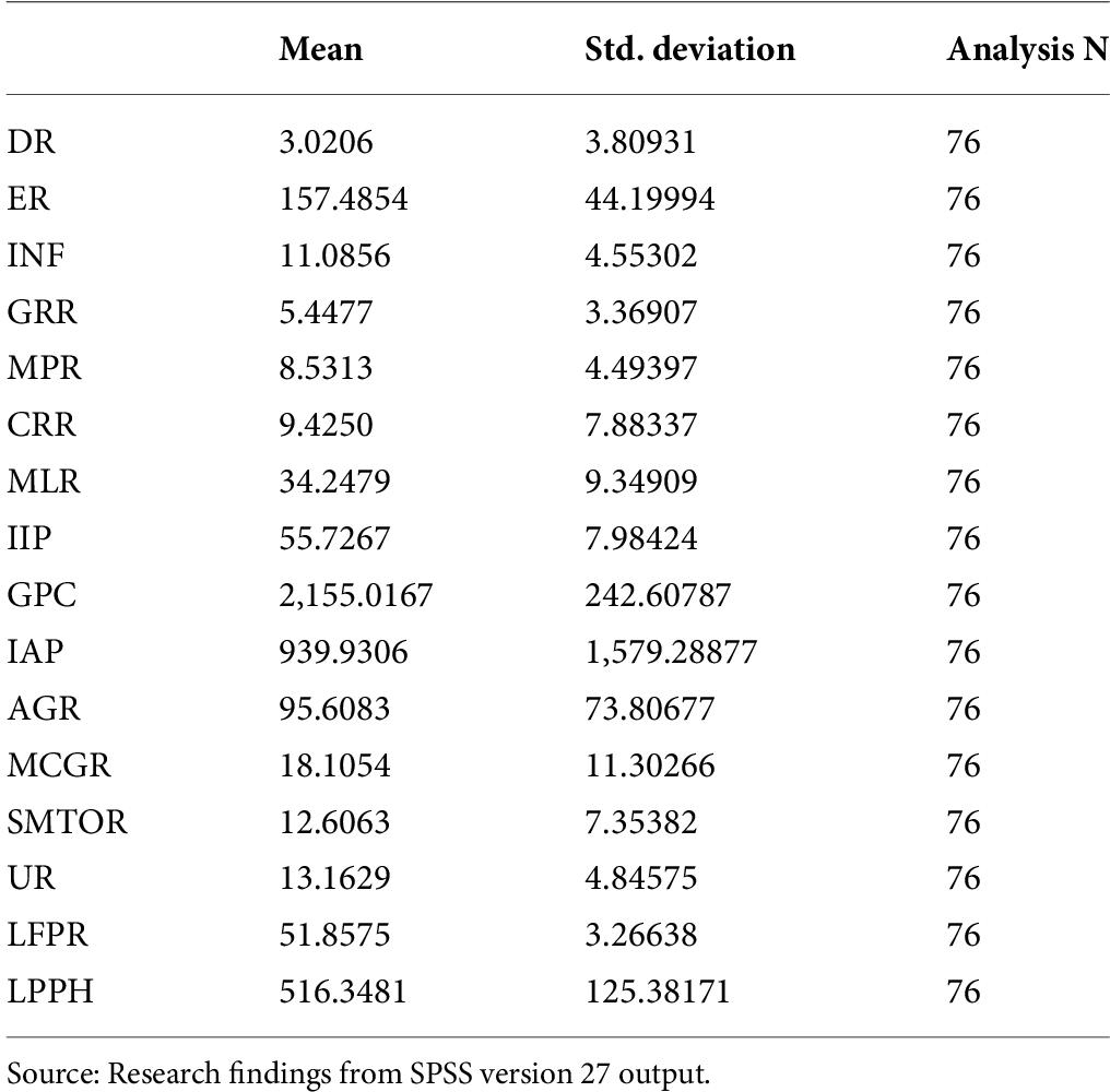
Table 1. Factor analysis descriptive statistics.
Test for sphericity and sampling adequacy
Table 2 indicates the Kaiser-Meyer-Olkin (KMO) and Bartlett’s tests. Bartlett’s test measures sphericity. The KMO Measure of Sampling Adequacy, below 0.5, is considered poor, and above 0.5, preferably above 0.6, is taken as a properly correlated identity matrix, eliminating the challenges of multicollinearity. The significance of 0.000 indicates that the model is properly fitted and the factors load perfectly. The p-value is less than 0.001, which is normal, but by default SPSS reports p-values less than 0.001 as 0.000. The Approx. Chi-Square statistic measures the adequacy of the number of observations (N); values above 220 are said to be normal. However, ours is 972.939, which portrays that the adequacy of the number of observations is very high.
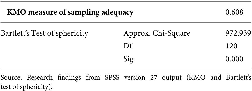
Table 2. Kaiser-Meyer-Olkin (KMO) and Bartlett’s test.
Communalities
Communalities, as shown in Table 3, represent the total influence of the observed variables possessed on predictive. This statistic is akin to the sum of the entire squared factor loading to the observed variable (the same as R2 in multiple regression). The decision criterion implies that extracted communality values range from 0 to 1, where 1 indicates that the variable is fully defined by the factors. In contracts, values tending towards 0 indicate that the variable cannot be predicted from any of the factors.
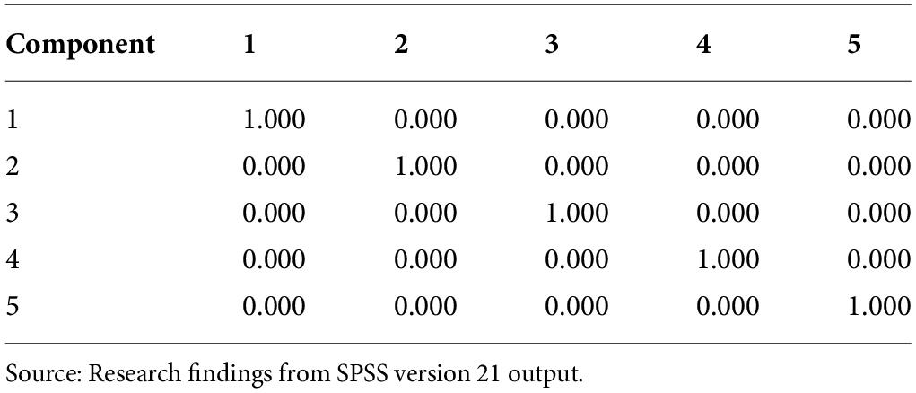
Table 3. Component score covariance matrix.
As shown in Table 4, the predictive factor, DR, has a commonality extraction of 0.677, while the other explanatory variables have shown very high commonality extractions of 0.059 for LPPA, 0.973 for GPC, 0.963 for IPP, 0.944 for cash reserve ratio (CRR), 0.910 for market capitalizations to gdp ratio (MCGR), 0.928 for minimum liquidity ratio (MLR), 0.918 for AGR, which are very close to 1, meaning that the observed variables are fully defined by the factors.
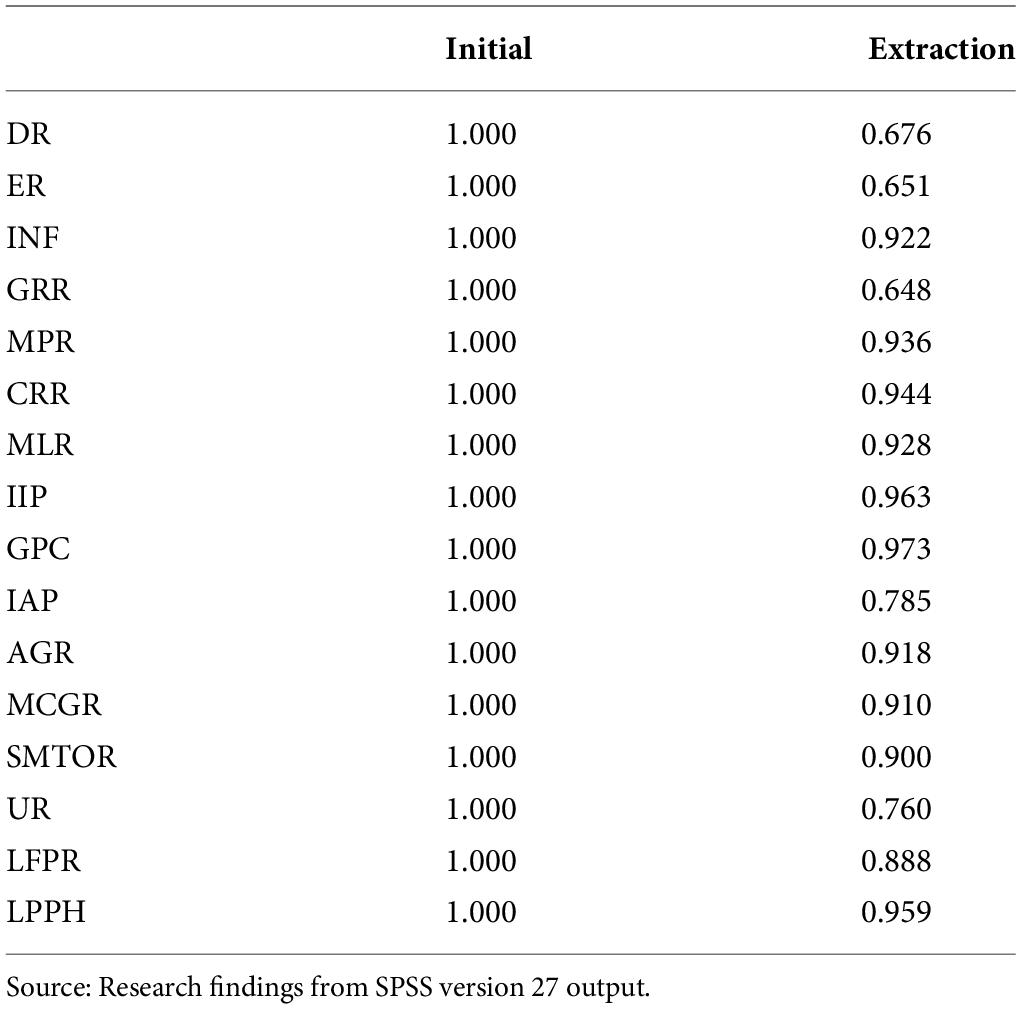
Table 4. Communalities.
Total variance
The variability in the data is explained by the total variance that the extracted factors have modeled. From the Variance Table 5, we have five (5) factors/components with an Eigenvalue greater than 1.00 that explain 85.997% of the cumulative variability in the data. This leads to the conclusion that a five-factor solution will be ideal for the study.
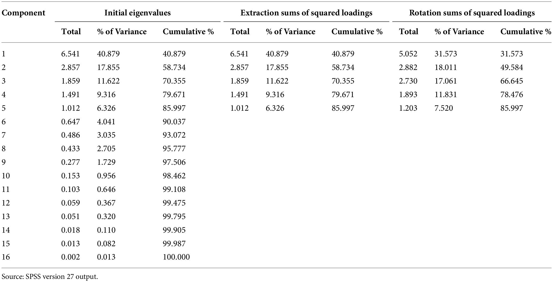
Table 5. Research findings from extraction method: principal component analysis (PCA).
In detail, Factor 1 accounts for 40.879% of the variability, Factor 2 harbors 17.855%, Factor 3 holds 11.622%, Factor 4 has 9.316%, and Factor 5 takes the least of 6.326.
Scree plot
The scree plot as seen in Figure 1 also helps to show where the factors leveled off using an eigenvalue greater than 1. The scree plot above helps to determine that five factors are all above the eigenvalue of 1 on the graph, thereby indicating that the factors are properly extracted and also adequate in modeling the dynamics of DR on the factors. Following the factor analysis carried out using the PCA method, the screen plot as seen in Figure 1.
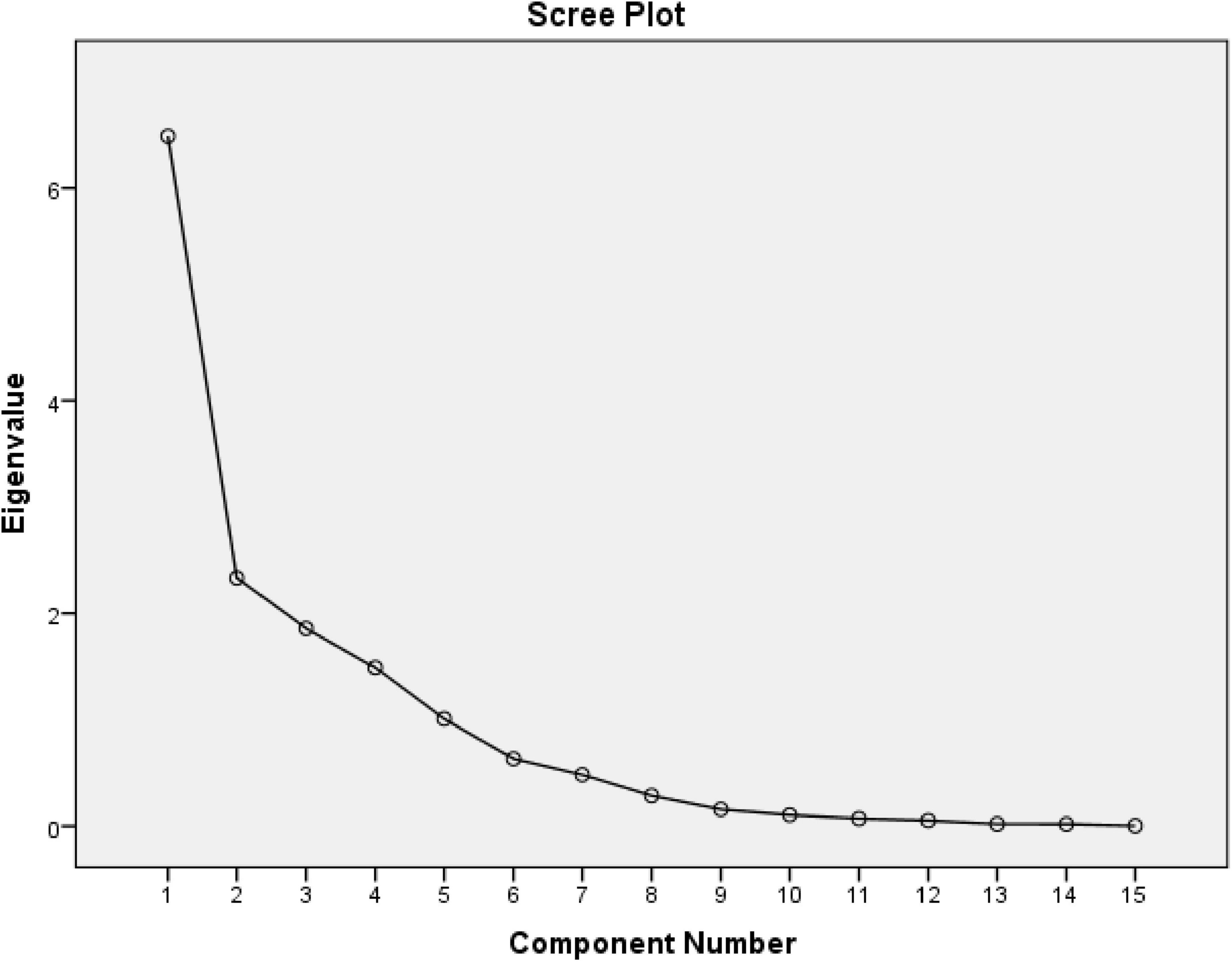
Figure 1. Scree plot. Source: SPSS version 21 output.
Factor loadings
The principal component criterion is applied when choosing the number of variables under the five various factors. The extraction of factors using the PCA (to aid in extracting uncorrelated linear combinations of variables) and rotation through the Varimax to help simplify the factors. All adequately have a component score coefficient above 0.05%.
Table 6 showed that the five factors were conveniently loaded/extracted for the study under query. Under the DFA, the predictive variable is the first component, while the proceeding components are the explanatory variables. The predictive component, DR, helps indicate a positive or negative relationship with other variables. As a general rule of thumb, only variables with the highest positive loading will be selected as the respective factor variables.
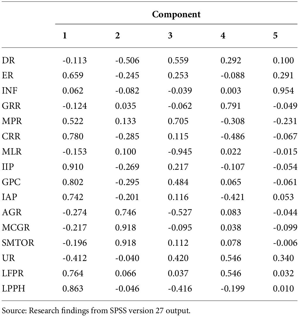
Table 6. Rotated component matrix.
Originally, it was expected that the fifteen explanatory variables under study would conveniently and evenly load under macroeconomic, banking regulation, stock market, business cycle, and labor market factors, given their idiosyncratic/individualistic latent characteristics. However, upon further query of the rotated component matrix, it was discovered that some labor market and macroeconomic factor variables behaved towards the business cycle. INF moved away from macroeconomics to assume the price changes indicator, while the entire Labor market behaved strangely by eliminating itself to assume latent behavior about the business cycle and macroeconomics. This dynamic caused a realignment of explanatory variables along their idiosyncratic traits. The latent combinations are shown below.
Factor identification and relationship with default rate
Factor 1 is identified as the Business Cycle Factor. The highest positive loadings are 0.910, 0.863, 0.802, 0.780, 0.764, 0.742, and 0.695, respectively corresponding to index of industrial production (IIP), labor productivity per hour (LPPH), GPC, CRR, LFPR, IAP, and ER. The lead indicator is IIP, which is an indicator of the business cycle. Other variables following the IIP seem to possess similar latent factors that depict why they queue behind the lead variable.
Therefore, Factor 1 possesses an overall variability of 40.876%, which is negatively related to the predictive variable, DR. In other words, each variable loaded under Factor 1 has a negative relationship with the dependent variable, simplifying an inverse relationship. This implies that an increase in explanatory variables will lead to a decrease in predictive variables and vice versa.
The negative relationship between the DR and factor 1 (business cycle factor) is expected and in line with the Austrian Business Cycle Theory. This incidence is equally typical of the Nigerian economy, where the financial institutions grant more credit during economic recession to stimulate the economy and, in turn, its side effect of the high DR.
Factor 2 is identified as the Stock Market Factor that accommodates three positive loadings at a 5% significance level. The loadings are MCGR, stock market turn over ratio (SMTOR), AGR, and MLR with the corresponding rotated loading component matrix of 0.918, 0.918, 0.746, and 0.100. The lead variable under this factor is related to the stock market. Hence, Factor 2 can be termed the Stock Market Factor. The individual variable under this factor reflects a negative relation with the first principal component, the predictive variable, and the DR. The overall explanatory power of Factor 2 is 17.655%. Variables under Factor 2 have a negative relationship with the predictive variable. Economically, this outcome is expected and typifies what happens in the Nigerian economy, where a downward or low-performing stock market will instigate high DRs in the Nigerian banking sector.
Factor 3 is identified as the Banking Regulation Factor. This factor assumes a positive relationship with the predictive variable, DR. Only the MPTR with the rotated component matrix of 0.705 loaded. The MPR fashion after a Banking Regulator’s latent behavior is hence tagged a Banking Regulation Factor. The variable under this Factor is significant at 5% because it single-handedly accounts for a variability of 11.622%, indicating the strength of the MPR in possessing idiosyncratic traits of the Banking Regulator Factor.
The positive relationship is a reflection of the Nigerian economy as it patterns to banking regulatory actions/policies. Ultimately, it aligns with Economic Theory. More so, the higher the MPR, the more defaults it creates.
Factor 4 is identified as a Macroeconomic Factor that has idiosyncratic characteristics of the Macroeconomy harboring GRR and UR with a positive factor loading of 0.791 and 0.546, respectively. Hence, it is called Macroeconomic Factor. Its variability of 9.316% is significant at 5%. The variables under this factor have a positive relationship with the predictive variable. Though this relationship is not expected, it is in line with economic theory, and scholars are linking loan portfolio credit with macroeconomic factors. Their studies establish that default risk tends to rise during economic downturns. However, banks with higher non-performing loans are those with more exposures to the macroeconomic risks.
Factor 5 is known as the Price Indicator Factor. It has a latent trait that tends towards price indicators. Hence, it is labeled the Price Indicator Factor. It accounts for 6.326% variability and has a positive relationship with the predictive variable, DR. Though not significant at the 5% level.
Test for the Significance of the Factor Loadings (Hypotheses)
According to Koutsoyiannis (91), it is assumed that the loadings are in effect similar to the correlation coefficients, so the test for significance of the factor loadings in PCA, as shown in Table 7, is done based on their levels of significance of the Pearson correlation coefficients. The Pearson Product Coefficients have critical values for the significance of different sample sizes (number of observations). These critical values are the standard errors of the Pearson Product Coefficient. The number of observations in this study is 76. If the value of the predictive variable at a 5% level of significance is greater than ± 0.280, then it is statistically significant. On the contrary, it will be regarded as statistically insignificant.
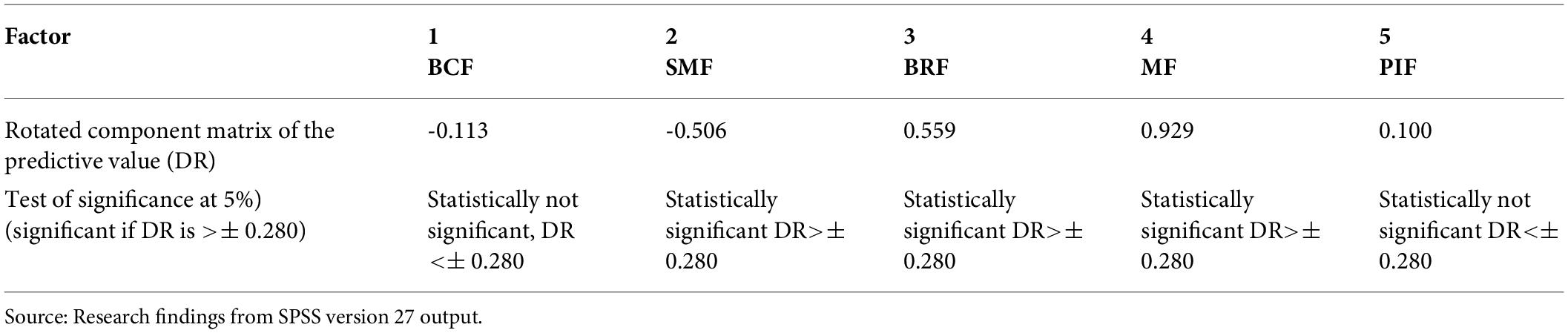
Table 7. Hypotheses testing of factor loadings.
The following hypotheses with their results are summarized: The relationship between the DR and the Business Cycle Factor is not significant; however, this relationship is negative. The relationship between the DR and Stock Market Factor is also negative and also statistically significant. There is a positive and statistically significant relationship between the DR and the Banking Regulation Factor. The relationship that exists between the DR and Macroeconomic Factor is positive and statistically significant, and there is no significant relationship between DR and Price Indicator Factor. However, the relationship is positive.
Discussion of results
In applying the DFM, we discovered that there are five common factors underscoring the DR in the Nigerian banking industry. These five factors account for 85.997% of the variability in the default of credit portfolios. This implies that 85.997% variability of DR is not due to individual idiosyncratic customer/bank factors but based on common factors that impact the broader banking industry. We can say that if 85.997% of the variability of the DR is common to the banking industry, then the spread of such a default is high and could cause a contagion defaulting effect on the larger economy. On the other hand, such signs of high default signal for measures to be taken against defaulting.
Factors were extracted using the PCA and rotated through varimax rotation to help simplify the factors. Upon the five factors extracted, Factor 1 accounts for 40.8997% of variability, Factor 2 harbors 17.855%, Factor 3 holds 11.622%, Factor 4 has 9.316%, and Factor 5 takes the least, 6.326%.
Originally, it was expected that fifteen explanatory variables under the study would conveniently and evenly load under the macroeconomic, banking regulation, stock market, business cycle, and labor market factors, given their idiosyncratic/individualistic latent characteristics. However, upon examining the rotated component matrix (of factor analysis), it was discovered that some labor market and macroeconomic factor variables tended towards the business cycle, while INF moved away from macroeconomics to assume the price changes indicator.
Entirely, labor market factors behaved strangely by eliminating themselves to assume the latent behavior of the business cycle and macroeconomic factors. The explanatory variables encountered realignment by these dynamics with their idiosyncratic traits.
Factor 1 associated variables loaded as the business cycle. This business cycle factor has a negative relation to the predictive variable and accounts for 80.876% variability in the DR, though the relationship is not statistically significant. However, it agrees with the Austrian business cycle theory, and the relationship is typical of the Nigerian economy, in the sense that financial institutions grant more credit during the recession to stimulate the economy and, in turn, bra high DR.
Factor 2, related variables loaded as a stock market factor, has a negative relationship with the DR, accounting for 17.655% variability. The statistically significant negative relationship typifies that a low-performing stock market will cause a rise in the DR. The result is confirmed by the present state of the Nigerian stock market, just as the relationship is expected. The escalation of default has arisen because of the downturn of the Nigerian stock market.
Factor 3 variables loaded as banking regulation factors with a statistically positive relationship with the DR. MPR is the leading variable that single-handedly accounts for a variability of 11.622%, indicating strength. The positive relationship is a reflection of the Nigerian economy as it pertains to banking regulatory actions and policies. More so, the higher the MPR, the more defaults it creates.
Factor 4, loaded as a Macroeconomic factor, has idiosyncratic characteristics of the macroeconomy, housing the GRR and UR, and having positive factor loadings of 0.791 and 0.546, respectively. Its variability is 9.3163% with a significance level of 5%. This relationship is not expected, but it is in line with economic theory.
Factor 5 is loaded as a Price Indicator Factor, and it accounts for 6.326% with a positive but not significant relationship with the DR. The study result is expected, and it conforms to economic theory, bearing in mind that inflationary pressures could propel defaults of banks’ credit portfolios without the institutionalizing of control measures.
Conclusion
In this research, we modeled credit default in the Nigerian Banking Sector using DFA against business cycle, macroeconomics, banking regulation, stock market, and labor market factors. In the modeling, we framed this research after the works of Cipollini and Missaglia (32); Jakubik (93); Duan and Miao (1); Hamerle et al. (94); Lamb and Perraudin (30, 31); Koopman et al. (33, 95); Senkoto (5); Kattai (6); and Tudela and Young (40). The results summarily indicate that Stock Market Factors, Banking Regulatory Factors, and Macroeconomic Factors are significant and help determine common patterns or contributing factors that determine default in the Nigerian Banking Industry.
Recommendations
To strengthen and ensure financial stability in the banking sector, the study recommends the full implementation of Basel III, as it will help create capital buffers beyond the minimum requirements and tackle procyclical effects in times of economic boom. Liquidity and stock market efficiency tactically reduce defaults, which is premised on the fact that banking and stock market activities have a positive, complementary impact on economic growth. The financial regulatory authorities, including the Monetary Policy Committee, should strengthen monetary policies and strive to achieve a single-digit Monetary Policy Rate and related variables.
Author contributions
EMS: Conception and design of study, Acquisition of data, Analysis and/or interpretation of data, Drafting the manuscript, Others corrections. JIKN: Conception and design of study, Analysis and/or interpretation of data, Drafting the manuscript, Critical review and revision, Others corrections.
Funding
There is no funding or grant for this publication.
Conflict of interest
The authors declare that the research was conducted in the absence of any commercial or financial relationships that could be construed as a potential conflict of interest.
References
1. Duan J, Miao W. Default correlations and large-portfolio credit analysis. J Bus Econ Stat. (2016) 34(4):536–46.
2. Jakubik P. Macroeconomic determinants of industrial default rates of Chinese enterprises. BOHR Int J Fin Market Res. (2007).
3. Cont R, Deguest R, Tankov P, Applebaum D, Kallsen J, Eberlein E. Modelling credit risk with Lévy and poisson processes. Q Financ. (2011) 11(4):493–512.
4. Chatterjee S. Modeling Credit Risk. Handbook – No.34. London: Centre for Central Banking Studies, Bank of England (2015).
5. Senkoto N. Macroeconomic variable underlying synchronization in probability of default of South African companies. Unpublished Dissertation, University of Johannesburg (2012).
6. Kattai R. Credit risk model for the Estonian banking sector. Working Paper Series. Eesti Pank Bank of Estonia (2010).
7. Mason SP, Bhattacharya S. On the optimality of asset-backed securities. J Math Econ. (1995) 24(3):301–21. doi: 10.1016/0304-4068(94)00701-3
8. Jarrow R, Turnbull S. Pricing derivatives on financial securities subject to credit risk. J Finance. (1995) 50(1):53–86.
9. Merton RC. On the pricing of corporate debt: the risk structure of interest rates. J Finance. (1974) 2:449–71.
10. Black F, Scholes M. The pricing of options and corporate liabilities. J Polit Econ. (1973) 81(3):637–54.
11. Geske R. The valuation of corporate liabilities as compound options. J Financ Quant Anal. (1977) 12(4):541–52. doi: 10.2307/2330330
13. Black F, Cox JC. Valuing corporate securities: some effects of bond indenture provision. J Finance. (1976) 31:351–67.
14. Turnbull SM. Probability of default of firms’ assets and liabilities. J Bank Fin. (1979) 3(2):149–64.
15. Geweke J. The dynamic factor analysis of economic time series. In: Aigner DJ, Goldberg AS editors. Latent Variables in Socio-Economic Models. Amsterdam: North-Holland Publishing Company (1977).
16. Sargent TJ, Sims CA. Business cycle modeling without pretending to have too much a-priori economic theory. In: Sims CA editor. New Methods in Business Cycle Research. Minneapolis: Federal Reserve Bank of Minneapolis (1977).
17. Bai J, Ng S. Determining the number of factors in approximate factor models. Econometrica. (2002) 70(1):191–221.
18. Stock JH, Watson MW. Forecasting using principal components from a large number of predictors. J Am Stat Assoc. (2006) 101(476):1167–79.
19. Upper C, Worms A. Estimating bilateral exposures in the German interbank market: Is there a danger of contagion? Discussion Paper 09/02. Economic Research Centre of The Deutsche Bundesbank (2002).
20. Gropp R, Vesala J. Deposit insurance, moral hazard and market discipline: evidence from Europe. N Am J Econ Fin. (2004).
21. Brasili A, Vulpes G. Co-movements in banking risk: an analysis for the Italian banks. J Bank Fin. (2005) 29(8–9):1975–94.
22. Stock JH, Watson MW. Dynamic factor models. In: Clements MP, Hendry DF editors. Oxford Handbook of Economic Forecasting. Oxford: Oxford University Press (2010).
23. Forni M, Hallin M, Lippi M, Reichin L. The generalized dynamic factor model: identification and estimation. Rev Econ Stat. (2000) 82:540–54.
24. Forni M, Hallin M, Lippi M, Reichin L. The generalized dynamic factor model: one-sided estimation and forecasting. J Am Stat Assoc. (2005) 100(471):830–40.
26. Gropp R. Fragility indicators for European credit risk portfolios. J Bank Fin. (2006) 30(8):2223–45.
27. Lehar A. Measuring systemic risk: a risk management approach. J Bank Financ. (2005) 29(10):2577–603. doi: 10.1016/j.jbankfin.2004.09.007
28. Nickell P, Perraudin W, Varotto S. Ratings Versus Equity-Based Credit Risk Modelling: An Empirical Analysis (Bank of England Working Paper No. 132). Bank of England (2001). Available online at: https://www.bankofengland.co.uk/working-paper/2001/ratings-versus-equity-based-credit-risk-modelling-an-empirical-analysis
29. Sanusi LS. The Nigerian banking industry: what went wrong and the way forward. Convocation Lecture Delivered at Bayero University, Kano. Central Bank of Nigeria (2010).
30. Lamb R, Perraudin W. Dynamic loan loss distributions: estimate and implications. Imperial College Working Papers, London. Imperial College London (2006).
31. Lamb R, Perraudin W. Dynamic default rate. Imperial College Working Papers: TBS/RML/WP II. Imperial College London (2008).
32. Cipollini A, Missaglia G. Dynamic Factor Analysis of Industry Sector Default Rates and Implications for Portfolio Credit. University of Essex, Department of Accounting, Finance, and Management (2007).
33. Koopman SJ, Lucas A, Schwaab B. Dynamic factor models with macro, frailty, and industry effects for U.S. default count: the credit crisis of 2008. Working Paper Series No 1459. ECB (2012).
34. Sy W. A Transition Matrix Model of Credit Risk. Australian Prudential Regulation Authority (2007).
35. Kim J. Conditioning on systematic factors: a cash flow theory of default. J Fin Econ. (1999) 53(1):3–32.
36. Scott J. The probability of bankruptcy: a comparison of empirical predictions and theoretical models. J Bank Financ. (1981) 53:317–44. doi: 10.1016/03784266(81)90029-7
37. Zeitun R, Benjelloun H. The efficiency of banks and financial crisis in a developing economy: the case of Jordan. Int Rev Account Bank Financ. (2012) 4:28–60.
38. Nickell P, Perraudin W. How much bank capital is needed to maintain financial stability? Bank of England Working Paper, Mimeo. Bank of England (1999).
39. Lehar A. Implementing a Portfolio Perspective in Banking Supervision. Mimeo: University of Vienna (2003).
40. Tudela M, Young G. A Merton-model approach to assessing the default risk of UK public companies. The Bank of England Working Paper No.194. Bank of England (2003).
41. Nilson B, Laurin M, Martynenko O. The Influence of Macroeconomic Factors on the Probability of Default: A Study of the Relationship Between Default Probabilities and Macroeconomic Variables. Unpublished Thesis, Lund University (2009).
42. Koopman SJ, Lucas A, Monteiro A. Credit cycle and macro fundamentals. J Empir Finance. (2009) 16:42–54.
43. Shahnazarian H, Sommar PA. Macroeconomic Factors and Probability of Default: A Study of Swedish Corporate Sector. Sveriges Riksbank Working Paper Series. Sweden: Sveriges Riksbank (Central Bank of Sweden) (2008). p. 216.
44. Rolwes K, Simons D. Credit risk and macroeconomic influences: evidence from credit default swaps. J Bank Fin. (2008) 32(9):1881–91.
45. Jimenez G, Mencia J. Modelling the distribution of credit losses with observable and latent factors. J Empir Finance. (2009) 16:42–54.
46. Dionne G, Harchaoui TM. Banks’ capital, securitization and credit risk: an empirical evidence for Canada. Insurance Risk Manag. (2008) 75(4):459–85.65bc.
47. Bonfim D. Credit risk drivers: evaluating the contribution of firm level information and macroeconomic dynamics. J Bank Fin. (2009) 33(2):281–99.
48. Qu Y. Macroeconomic factors and probability of default. Eur J Econ Finance Admin Sci. (2008) 13:192–215.
50. Galai D, Masulis RW. The option pricing model and the risk factor of stock. J Financ Econ. (1976) 3(1–2):53–82. doi: 10.1016/0304405X(76)90020-93000
51. Denis DJ, Denis DK. Causes of financial distress following leveraged recapitalizations. J Financ Econ. (1995) 37(2):129–57.
54. George TJ, Hwang C. A resolution of the distress risk and leverage puzzles in the cross-section of stock returns. J Financ Econ. (2010) 96:56–79.
57. Loughran T, Ritter JR. The new issues puzzle. J Financ. (1995) 50(1):23–51. doi: 10.1111/j.1540-6261.1995.tb05166.x2d28
59. Allen F, Gale D. Optimal currency crises. Carnegie-Rochester Conf Ser Public Policy. (2000) 53(1):177–230.
62. Allen F, Gale D. Financial intermediaries and markets. Econometrica. (2004) 72(4):1023–61. doi: 10.1111/j.1468-0262.2004.00525
64. Maddaloni A, Peydro JL. Monetary policy, macroeconomic conditions, and credit risk. J Bank Fin. (2013) 37(8):3047–61.
65. Bhamra HS, Fisher AJ, Kuehn LA. Monetary policy and corporate default. J Monet Econ. (2010) 58(5):480–94.
67. Kashyap AK, Stein JC. The optimal conduct of monetary policy with overlapping generations. J Monet Econ. (2010) 57(2):181–94.
68. Maddaloni A, Peydró JL. Bank risk-taking, securitization, supervision, and low interest rates: evidence from the Euro-area and the U.S. lending standards. Rev Financ Stud. (2011) 24(6):2121–65. doi: 10.1093/rfs/hhr015
69. Ciccarelli M, Maddaloni A, Peydró JL. Trusting the Bankers: A New Look at the Credit Channel of Monetary Policy [Working Paper]. European Central Bank (2011).
70. Gonzalez-Aguedo C, Suarez J. Interest rates and credit risks. J Money Credit Bank. (2012) 47(23):445–80.
71. Jacobson T, Lindé J, Roszbach K. Firm Default and Aggregate Fluctuations (Working Paper No. 226). Sweden: Sveriges Riksbank (2011).
72. Ekpete MB, Okpala CS, Okoli MN, Nwankwo OC, Eze PO, Udo IE. Credit risk and macroeconomic influences: evidence from Nigerian banks. J Econ Sustain Dev. (2019) 10(2):1–13. doi: 10.7176/JESD/10-2-01
73. Favilukis J, Lin X, Zhao X. The elephant in the room: The impact of labor obligations on credit risk. Econometric World Society Congress. (2016).
74. Zhang L, Hu H, Zhang D. A credit risk assessment model based on SVM for small and medium enterprises in supply chain finance. Financ Innovat. (2015) 1(1):1–21. doi: 10.1186/s40854-015-0014-5
75. Favilukis J, Lin X. Wage rigidity: a quantitative solution to several asset pricing puzzles. Rev Financ Stud. (2015) 28(1):148–182.
76. Berk F, Walden J. Limited capital market participation and human capital risk. Rev Asset?Pricing Stud. (2013) 3:1–37.
77. Bansal R, Yaron A. Risks for the long run: a potential resolution of assets pricing puzzles. J Finance. (2004) 59:1481–509.
79. Allen F, Gale D. Financial fragility, liquidity, and asset prices. J Eur Econ Assoc. (2002) 2(6):1015–1048.
80. Jhingan ML. Money, Banking, International Trade and Public Finance. Delhi: Vrinda Publications Ltd (2011).
81. Kindleberger C. Manias, Panics, and Crashes: A History of Financial Crises. New York: Basic Books (1978).
82. Diamond D, Dybvig P. Bank runs, deposit insurance, and liquidity. J Polit Econ. (1983) 91:401–19.
83. Calomiris C, Mason J. Causes of U.S. bank distress during the depression. NBER Working Paper W7919. Cambridge, MA: National Bureau of Economic Research (2000).
84. Calomiris CW, Gorton G. The origins of banking panics: models, facts, and bank regulation. In: Hubbard RG editor. Financial Markets and Financial Crises. Chicago: University of Chicago Press (1991). p. 109–74.
85. Stock JH, Watson MW. New indexes of coincident and leading economic indicators. In: NBER Macroeconomics Annual. Vol. 4. Cambridge (MA): MIT Press (1989). p. 351–94.
86. Stock JH, Watson MW. Macroeconomic forecasting using diffusion indexes. J Bus Econ Stat. (2002) 20:147–62.
87. Stock JH, Watson MW. Forecasting using principal components from a large number of predictors. J Am Stat Assoc. (2002) 97:1167–79.
88. Stock JH, Watson MW. Dynamic factor models, factor-augmented vector autoregressions, and structural vector autoregressions in macroeconomics. In: Taylor JB, Uhlig H editors, Handbook of Macroeconomics (Vol. 2). Elsevier (2016). p. 415–525.
89. Ionota F, Schiopu I. Credit risk and macroeconomic influences: evidence from Romanian banks. J Bank Fin. (2010) 34(2):281–99.
90. Xu X, Chen J, Wang Y, Li H, Zhang L, Liu Z. Credit risk and macroeconomic influences: evidence from Chinese banks. J Bank Financ. (2010) 34(2):281–99.
92. Kaiser HF. The varimax criterion for analytic rotation in factor analysis. Psychometrika. (1958) 23(3):187–200.
93. Jakubik P. Macroeconomic determinants of credit risk: evidence from the Czech Republic. Czech J Econ Fin. (2009) 59(1):40–61.
94. Hamerle A, Liebig T, Scheule H. Forecasting credit portfolio risk. Deutsche Bundesbank Discussion Paper. Deutsche Bundesbank (2003).
95. Koopman SJ, Lucas A, Schwaab B. Forecasting Cross-Sections of Frailty-Correlated Default. TWinbergen Institute (2008).
© The Author(s). 2026 Open Access This article is distributed under the terms of the Creative Commons Attribution 4.0 International License (https://creativecommons.org/licenses/by/4.0/), which permits unrestricted use, distribution, and reproduction in any medium, provided you give appropriate credit to the original author(s) and the source, provide a link to the Creative Commons license, and indicate if changes were made.