1. Introduction-1452742568-1452742568
Diabetes is a chronic illness on the increase nowadays. It is classified as a noncommunicable disease (NCD) in this context since it is not transmissible from one person to another and is caused by a mix of genetics, physiology, environment, and behavior. When the body’s blood glucose levels are between 4.4 and 6.1 millimoles per liter, diabetes is said to be present. Insulin utilization is hampered by a diabetic’s decreased insulin secretion. There are four different forms of diabetes: Type 1, Type 2, Type 3, and Type 4.
Type 1 diabetes mellitus (T1D) is an autoimmune disease that leads to the destruction of insulin-producing pancreatic beta cells. When someone has type 2, their body either has trouble producing insulin or has trouble absorbing it. It often affects age-related demographics. Pre-diabetes is a Type 3 diabetes (1) illness characterized by raised blood sugar levels but not as high as Type 2 diabetes. Type 4 gestational diabetes most commonly affects pregnant women.
Symptoms: Polyuria is characterized by frequent urine, food cravings, excessive thirst, weight loss, sluggish wound healing, foggy vision, and feelings of weariness.
Diagnosis: The HBA1C test examines blood sugar levels over 3°months and can help predict Type 2 and Type 3 diabetes. The FPGT test predicts Type 2 diabetes by evaluating blood sugar levels following an 8°h fast. The oral glucose tolerance test, or OGTT, is used to diagnose Type 2 diabetes, pre-diabetes, and gestational diabetes.
Treatment: Diabetes is a chronic illness that cannot be cured but may be controlled with insulin, which comes in many forms, as well as a healthy diet, oral medications, and frequent exercise.
Diabetes affects 422 million people worldwide. Diabetes is expected to affect more than 60 million Indians out of a population of 135 billion. By 2035, this pitiful illness will have reached a staggering 109 million patients. According to the World Health Organization (WHO) (2), diabetes will be one of the seven leading causes of mortality by 2030. According to WHO research, approximately one-third of diabetic women are unaware of the dangers of the disease. Additionally, gestational diabetes increases the risk of disease transmission from pregnant women to their unborn offspring. Diabetes, a condition that may cause consequences such as abnormal pregnancies, renal failure, and vision loss, is an urgent issue that requires early identification and prevention. Machine learning, a burgeoning discipline of data science, employs algorithms and numerical models to enhance task performance by constructing a scientific model of sample data. The suggested study seeks to apply several machine learning classifiers for diabetes research, including KNN, NB, SVM, DT, RF Classifier, LR, GB, and ensemble learning. This will assist researchers in discovering new facts from health-related datasets and improving medical services, illness supervision, and disease prediction. The parameters of the PIDD dataset are utilized as inputs, and the optimal classifier for predicting diabetes in a patient is selected after a rigorous analysis.
1.1 Literature review
A literature survey was conducted to know the different models that we can use on our work. Table 1 shows an overview of our literature survey.
1.2. Dataset
The suggested models are tested using the Pima Indian Diabetes Dataset (PIDD) from UCI Machine Learning Repository is a collection of databases, University California Irvine (UCI).
This dataset has 2,000 entries with 8 attributes, with class outputs (0 and 1) representing diabetic patients and class 0 representing non-diabetic patients.
The attributes here are:
(i). Pregnancies
(ii). Body Mass Index (BMI)
(iii). Diabetes Pedigree Function (DPD)
(iv). Age
(v). Insulin
(vi). Glucose
(vii). Blood Pressure
(viii). Skin Thickness
2. Methodology
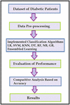
The proposed model (Figure 1) is structured for the analysis and evaluation of (PIDD). In our model, we first import the specified dataset. Then we use different data visualization techniques like:
• Histogram (to check frequencies of each parameter),
• Heatmap (to visualize the correlation between each parameter),
• Countplot (to see the frequencies of diabetic and non-diabetic data),
• Boxplot (to check if any outliers are there in the data) and
• Pairplot (to visualize the pairwise relationships between the parameters)
On the basis of the nature of data, we perform Data Pre-processing by removing the outliers in the data. Next, we divide the dataset into test and training datasets. Then we train the dataset individually on 7 different classification algorithms. These are:
Logistic Regression, SVM, K-Nearest Neighbors, Decision Tree, Naive Bayes, Random Forest, and Gradient Boost classifiers are used for data classification. Customized Ensemble Learning is then performed by combining these algorithms.
Finally, we evaluate the performance of each of the algorithms. The performance metrics we have used are:
Accuracy measure, ROC Score, F1 Score, Loss Function, Sensitivity, Specificity.
Lastly, we compare the analysis based on accuracy and obtain the final results.
3. Results or finding
3.1. Data Pre-processing
3.2. An overview of the dataset
There are in total 2,000 entries or data members with 8 trainable independent variables to be analyzed to predict 1 dependent variable, the Outcome. There are no null values.
Out of the 2,000 data points, 1,316 data points have “0” (that is diabetes negative) as the outcome and the remaining 684 data points have “1” as the outcome (that is diabetes positive). As shown in Figure 2.
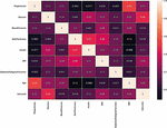
Figure 3 shows the correlation between the different attributes. It suggests that the data are not uniformly distributed or normalized. Age and pregnancies are inversely correlated, while skin thickness, insulin, and pregnancies are independent variables.
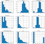
Figure 4 shows the histograms of the frequencies of data in all the attributes. The frequencies of the data for each attribute can be observed. It shows the regions where the maximum data points are present.
3.3. Outlier remove
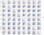
We have seen from Figures 5–8 that the attributes “Insulin,” “Blood Pressure,” and “Diabetes Pedigree Function” have some outliers present which need to be removed for uniform distribution and better performance. After removing the outliers, about 80 records got deleted and we get more uniform scattered matrix as shown in Figure 9.
3.4. Algorithms used in our work
We have done comparative studies and here are the algorithms used. We have used 7 machine learning classification models and 1 customized ensemble learning model for comparing the performances.
3.4.1. Logistic regression
When the aim is categorical, logistic regression, a powerful supervised machine learning technique, is used to address binary classification issues. A method for calculating the likelihood of a discrete output given an input variable is logistic regression. Logistic regression may be used as an analytical method to evaluate which category a new sample most closely resembles when dealing with classification problems.
The “maximum likelihood estimation (MLE)” loss function, a conditional probability, is used in logistic regression. A forecast is categorized as a class 0 prediction if its probability is greater than 0.5. If not, Class 1 will be chosen. The S-shaped sigmoid function in Figure 10 shows real values between [0, 1].

Figure 10. Sigmoid function (7).
3.4.2. Support vector machine (SVM)
Support vector machine (SVM) is a supervised learning technique for classification and regression in linear and nonlinear data. It generates a hyper plane in high- or infinite-dimensional space, dividing data into two classes for classification or regression. Support vectors are data points close to the hyper plane.
3.4.3. K-nearest neighbors (KNN)
K-nearest neighbor is a simple supervised machine learning algorithm used for classification and regression problems. It uses a non-parametric approach, making no assumptions about underlying data. KNN is a lazy learner, saving the dataset and using it to execute actions when classifying data, rather than learning from the training set immediately.
3.4.4. Decision tree classifier
Decision Tree is a tree-structured classifier with internal nodes representing dataset attributes, branches for decision rules, and leaf nodes for results. It provides a graphical representation of potential solutions to problems based on given conditions. Decision trees mimic decision-making, making them easy to understand.
3.4.5. Random forest
Random Forest is a supervised learning machine method used for classification and regression issues. It is based on Ensemble Learning, which merges multiple classifiers to solve complex problems and improve model performance. Random Forest uses multiple decision trees on different dataset subsets, averaging results to increase predicted accuracy and avoid over-fitting.
3.4.6. Naive Bayes classifier
The phrase “Naive Bayesian” refers to a classification approach based on the Bayes hypothesis that employs autonomous assumption amongst various indicators. The approach that employs the dataset as information performs research and predicts the grade using Bayes’ Theorem. It is typically used in high-dimensional training data-based text classification. It is referred to as naïve because it assumes that the presence of some characteristics is independent of the presence of other characteristics. Naive Bayes is frequently used in spam filtering, sentiment analysis, and article classification.
Here, P(A| B) is a posterior probability, that is probability of hypothesis A on observed Event B. P(B| A) is Likelihood Probability, that is probability of evidence given that probability of hypothesis is true.
3.4.7. Gradient boosting classifier
Gradient boosting is a machine learning method that improves weak learners by fixing the error of its predecessor. It uses residual errors from the predecessor as labels, unlike AdaBoost, which changes the training sample weight. Gradient Boosting involves three elements:
(i). A loss Function to be optimized.
(ii). A weak learner to make predictions.
(iii). An Additive Model to add weak learners to minimize the loss function.
3.4.8. Ensemble learning
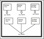
Ensemble learning is a general meta-approach to machine learning that seeks better predictive performance by combining the prediction from multiples models as in Figure 11. The reason why Ensemble Learning is efficient is that the machine learning model might work differently. Each model might perform well on some dataset and not on others, but when we ensemble the models, they cancel out each other’s weakness. Ensemble learning helps in capturing most of the diverse signals, produces less incorrect predictions, reduces overfitting, and hence, helps increase performance.
3.5. Outputs of experiments
Sensitivity Calculation of the algorithms are shown in Table 2.
Specificity Calculation of the algorithms are shown in Table 3.
3.6. ROC-AUC curve showing performance of the algorithms
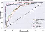
From Figure 12 it is observed that Decision Tree gives the maximum AUC value, which is equal to 0.939.
3.7. Performance comparison of the algorithms
From Table 4 it is observed that Ensemble Learning gives the maximum Accuracy, maximum F1 Score, and minimum L1-Loss value. The maximum ROC Score is given by Decision Tree, Maximum sensitivity score by Random Forest, and Maximum specificity value by KNN. Figures 13–20 show Learning Curves of the algorithms, which display Accuracy scores.
3.8. Learning curves of the algorithms showing accuracy scores
3.9. Learning curves of the algorithms showing L1-Loss values
Figures 21–28 illustrates Learning Curves of the algorithms showing L1-Loss values.
3.10. Parameters considered for some algorithms
3.10.1. K nearest neighbors algorithm
For KNN algorithm, the value of K has been determined by iterating from 1 to 40 for optimal K value for which the loss value is minimum. We have found out that when K = 1, we have got the minimum error for this algorithm, that is 0.12. Here K cannot be equal to 0. Figure 29 illustrates K value Vs. Error rate graph for KNN Algorithm
3.10.2. Gradient boost algorithm
For Gradient Boost algorithm, there are 2 parameters on which the algorithm’s performance depends. They are the learning rate and n-estimators. We have kept the learning rate constant at 0.18 where maximum performance was obtained and iterated the n-estimators value from 10 to 200 for optimal value, i.e., for minimum error rate. It has been found that when the n-estimators value is equal to 180, the algorithm gives best performance, i.e., minimum error of 0.06. Figure 30 depicts n-estimators value Vs. error rate graph for GB Algorithm.
Bar graphs comparing various performances of the algorithms.
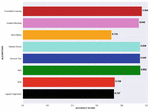
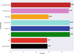
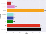
From Figure 31 it is observed that Ensemble Learning gives the maximum Accuracy score, which is equal to 0.964.
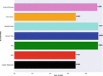
From Figure 32 it is observed that Decision Tree gives the maximum ROC score, which is equal to 0.939.
From Figure 33 it is observed that Ensemble Learning gives the maximum F1 score, which is equal to 0.940.
From Figure 34 it is observed that Ensemble Learning gives the minimum L1-Loss value, which is equal to 0.035.
3.11. Our web app for prediction
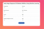
Finally, we have created a web app that takes the data attributes and inputs and finally predicts the output as “Diabetic” or “Non diabetic.” The predictions are shown individually by the 7 different algorithms. Figure 35 shows the homepage of our web application. It takes the attributes as inputs to a form.
We have used HTML5, CSS3, and Bootstrap 4 for designing the frontend.
We have used Flask framework and Python3 language for designing the backend of our web app.
Our web app has been hosted on the Heroku platform.
The link to our web app:
https://dmdiagnosisusingml.herokuapp.com/
Figure 36 demonstrates the Screenshot showing the prediction of a data point by the algorithms and Screenshot in Figure 37 showing the prediction of a data point by the algorithms.
4. Discussions
4.1. Discussion about uncertainty
When measuring a0 on a measured a∈(−∞,∞) with true value a*, the error e = |a* – a0| is often due to measurement inaccuracy. Uncertainty quantifies doubt about the measurement result, and can be known or unknown, resulting in an uncertain measurement.
4.1.1. Types of uncertainties
Uncertainty sources include subjective and objective types, subjective uncertainty being subjective and objective uncertainty being objective, which cannot be assessed. These two can be further divided as shown in the following section.
4.1.2. Uncertainty
(I) Objective Uncertainty
• Epistemic: Uncertainty in estimated model parameters.
• Aleatoric: Noise in data measurement.
(II) Subjective Uncertainty
• Moral Uncertainty: Bias in Moral or evaluative matters.
• Rule Uncertainty: Treating the doubt about a rule.
4.1.3. Sources of uncertainties
Uncertainty in machine learning in medical data can arise from various sources, including positional, value, data manipulation, and algorithms processing. Machines and sensors use machines and sensors, causing positional uncertainty, while measuring procedures create value uncertainty. Data manipulation and techniques transforming data into models contribute errors, incompleteness, and parameter uncertainty. Models cannot precisely map reality, introducing uncertainty, and their definitions cannot be full, further complicating the accuracy of machine learning in medical data analysis. Addressing these challenges is crucial for machine learning’s usefulness in medical data analysis.
4.1.4. Need for uncertainty measurement and its quantification
Because of its promising outcomes in decision-critical sectors, machine learning has gained popularity. However, safe procedures must account for the process’s inherent ambiguity. ML models learn from data and generate predictions using extracted models, which are subject to noise and poor model inference. To establish trustworthy AI-based systems, it is critical to assess uncertainty in forecasts and avoid making judgements where there is a high degree of uncertainty.
5. Conclusion
This research uses seven machine learning algorithms and a specialized ensemble learning method to analyze illnesses like diabetes. On the PIMA Indian Dataset, simulations demonstrate that the ensemble learning approach performs better than individual classifiers. For the automated treatment of chronic diseases in the future, the simulation model can be expanded to different diseases. With deep learning tools like the Convolutional LSTM model and boosting methods like Adaptive Boosting and Extreme Gradient Boosting (XGBoost), the work may be further developed. Accuracy can be enhanced with ensemble learning customizations. The work may be applied to other datasets with various properties, and the dataset comprises medical data with uncertainty resulting from human interaction.
Author contributions
All authors contributed to the article and approved the submitted version.
Dataset
Dataset: PIMA Indian Dataset https://www.kaggle.com/uciml/pima-indians-diabetes-database
References
1. Healthline.What is Type 3 Diabetes? Available online at: https://www.healthline.com/health/type-3-diabetes#What-is-type-3-diabetes?
3. Rahman M, Islam D, Mukti R, Saha I. A deep learning approach based on convolutional LSTM for detecting diabetes. Comput Biol Chem. (2020) 88:107329.
4. Reddy DJ, Mounika B, Sindhu S, Pranayteja Reddy T, Sagar Reddy N, Jyothsna Sri G, et al. Predictive machine learning model for early detection and analysis of diabetes. Mater Today Proc. (2020).
5. Lukmanto RB, Nugroho A, Akbar H. Early detection of diabetes mellitus using feature selection and fuzzy support vector machine. Procedia Comput Sci. (2019) 157:46–54.
6. Gillmann C, Saur D, Scheuermann G. How to deal with uncertainty in machine learning for medical imaging? Proceedings of the 2021 IEEE Workshop on TRust and EXpertise in Visual Analytics (TREX). New Orleans, LA: IEEE (2021). p. 52–8.
7. k2analytics.Introduction to Logistic Regression. Available online at: https://www.k2analytics.co.in/introduction-to-logistic-regression/

