Bohr article

Introduction

Scheduling is the allocation of resources to perform a collection of tasks over a period of time. Scheduling problems determine the order or sequence for processing a set of jobs through several machines in an optimal manner. Flow shop scheduling (FSS) problems consider m different machines and n jobs; each job consists of m operations, and each operation requires a different machine, and all the jobs are processed in the same processing order.

The problem to be solved is a FSS problem with the assumption that the orders are ready at the start of the scheduling process. The objective of the problem is to minimize the total weighted tardiness of orders. The constraints are on the sequence of orders, on the sequence of operations in the orders, and on machine changeover time.

The model of the problem is built based on the above assumptions, objective, and constraints. The genetic algorithm and tabu search (GATS) algorithm is built based on the combination of genetic algorithm (GA) and tabu search (TS) with the foundation of GA. Based on the model of the problem, the GATS algorithm will find a good solution for the problem; this solution will be compared with the solution of the currently used heuristic model to evaluate the effectiveness of the algorithm.

Literature review

FSS problems are nondeterministic polynomial (NP)-hard combinatorial optimization problems. For such problems, heuristics play a major role in searching for near-optimal solutions. Etiler et al., developed a genetic algorithm-based heuristic for the flow shop scheduling problem with makespan as the criterion (1). Complex GA algorithms have also been researched to solve the FFS problem effectively. Engin et al., developed an efficient GA for hybrid flow shop scheduling with multiprocessor task problems (2). Phong et al., developed a GA model to solve a flow shop scheduling problem, with the objective to reduce total weighted tardiness time and a constraint on changeover time in operations (3). Pezzella et al., developed a GA for the flexible job-shop scheduling problem. The algorithm integrates different strategies for generating the initial population, selecting the individuals for reproduction, and reproducing new individuals (4).

Gupta et al., designed a heuristic model based on TS for a two-stage flow shop problem (5). Phong et al., developed a TS model for a FSS problem (6). Burduk et al., applied TS and GA to solve production process scheduling problems (7). Umam et al., combined the TS process with a GA to solve the flow shop scheduling problem with the objective of minimizing makespan (8). Ben-Daya and Al-Fawzan proposed a TS approach for solving the permutation flow shop scheduling problem. The approach suggested simple techniques for generating neighborhoods of a given sequence and a combined scheme for intensification and diversification (9).

Phong et al., considered a pilot FSS problem with four different machines and 10 different jobs. The problem was solved by two different hybrid meta-heuristic models, GATS (10) and TSGA (11). Phong et al., developed a hybrid meta-heuristic model to solve FFS problems with nine orders, scheduling on four stations. The problem had the objective to minimize the total tardiness time and the constraints on workstation set-up times and production batch sizes (12).

In general, there are many hybrid meta-heuristic models, and the former models are rather complicated. This research proposes a simple combination of GA and TS. In the algorithm, GA is used as the platform for global search, and TS is used to support GA in local search. GA diversifies the search by exploring the search space, and TS intensifies the search by exploiting the best solutions found.

In each iteration, GA generates the elite population from the current population by using selection operators and generates genetic populations from the elite population by using cross-over and mutation operators. Then TS generates the neighborhood population from the genetic population by using neighborhood operators. Finally, GA generates the next population from the current population, the elite population, and the neighborhood population by using replacement operators. The detailed research methodology is shown in the next section.

Research methodology

The FSS problem is a NP-hard problem with a large size of solution space. The methodology used in this research to solve the problem includes four phases:

1) Phase A: Construct the model of the FSS problem.

2) Phase B: Construct the GATS algorithm.

3) Phase C: Use the GATS algorithm to solve the pilot FSS problem.

4) Phase D: Use the GATS algorithm to solve the real FSS problem.

Phase A: construct the model of the FSS problem

In phase A, the model of the problem is formulated with the objective of minimizing the total weighted tardiness time and constraint on the sequence of orders, on the sequence of operations in the orders, and on machine changeover time. The FSS model has indexes, parameters, and variables as in Table 1.

TABLE 1

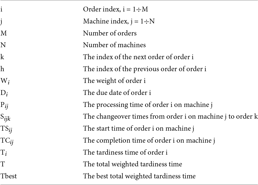
Table 1. The indexes, parameters, and variables of the FSS model.

In the case, there are four machines (N = 4), M₁, M₂, M₃, and M_4. Each order has three parts, P1, P2, and P3, processed in eight operations, O_j, j = 1÷8, distributed on the four machines as in Figure 1.

FIGURE 1

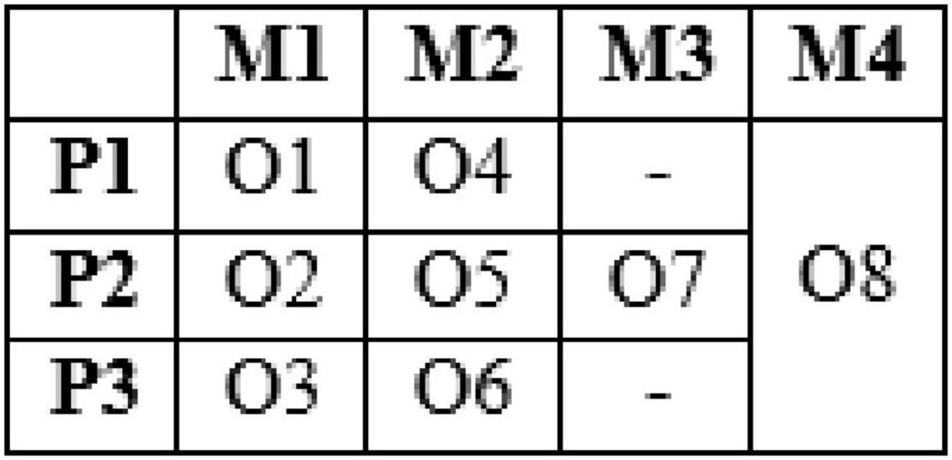
Figure 1. The production process.

The constraints on the sequence of operation on each order are as follows.

TS_i4 ≥ TC_i1,

TS_i5 ≥ TC_i2,

TS_i6 ≥ TC_i3,

TS_i7 ≥ TC_i5,

TS_i8 ≥ max(TC_i4, TC_i6, TC_i7).

The start time of order i at operation j, TS_ij depends on the completion time of the previous order h, TC_hj and the changeover time S_hji between the orders on operation j.

T S {}_{i j}= T C {}_{h j}+ S_{h j i}

The completion time of order i on operation j, TC_ij is determined by the start time and processing time of the order.

T C {}_{i j}= T S {}_{i j}+ P_{i j}

The tardiness time of order i, T_i is determined by the completion time of the last operation and due time of the order.

T {}_{i}= M a x (0, T C {}_{i 8}- D {}_{i})

The total weighted tardiness is defined as follows:

T = \sum_{i = 1}^{M} w_{i} T_{i}

The objective function that minimizes the total weight tardiness is defined as follows:

T b e s t = M i n T, T = \sum_{i = 1}^{M} w_{i} T_{i}

The model of the problem is summarized as follows:

Min T

St.

TS_i4 ≥ TC_i1,

TS_i5 ≥ TC_i2,

TS_i6 ≥ TC_i3,

TS_i7 ≥ TC_i5,

TS_i8 ≥ max(TC_i4, TC_i6, TC_i7).

TS_ij = TC_hj + S_hji

TC_ij = TS_ij + P_ij

T_i = Max (0, TC_i8 - D_i)

TS_ij, TC_ij ≥ 0.

Phase B: construct the GATS algorithm

The GATS algorithm combines GA and TS; GA is used to perform a global search of the solution space, and TS is used to perform a local search to refine the solution found by GA. The GATS procedure is as follows:

Step 1: Initialize the GATS model.

Step 2: Generate the initial population P⁽⁰⁾. Set k = 0.

Step 3: Generate elite population P_E^(k).

Step 4: Generate the genetic population P_G^(k).

Step 5: Generate the neighborhood population P_N^(k).

Step 6: Generate the next population P^(k+1). Set k = k+1.

Step 7: Check the termination rule. If No, return to step 3. If Yes, finish the loop.

Step 8: Run the algorithm a number of times to choose the best scheduling result.

Step 1: Initialize the GATS model

This step sets up the factors of GATS model, including:

- The method of coding

- The GA factors

- The TS factors

- The termination rule

- The number of runs

The method of coding: Schedule alternatives are coded by chromosomes. With N orders, each chromosome is a string of N genes. Each gene is corresponding to an order. The orders are numbered from 1 to N. The sequence of genes represents the sequence of order scheduled:

C = [G {}_{1}, G {}_{2}, \dots, G {}_{N}]

The GA factors: The GA factors include fitness function F, the population size P, and the parameters of GA operators. The GA operators include the following parameters:

- The selection method

- The crossover probability P_c

- The crossover method

- The mutation probability P_m

- The mutation method

- The replacement method.

In the GATS model, the fitness function F is defined as follows:

F {}_{i}= T {}_{m a x}- - T {}_{i}.

Where F_i, T_i are the fitness and objective values of chromosome i, T_max is the maximum objective value in the population.

The selection method uses selection probabilities, defined by fitness values, to choose chromosomes into the elite population. The crossover method is POX (Precedence Operation Crossover), the mutation method is SWAP, and the replacement method is acceptance threshold with threshold factor K.

The TS factors: The TS factors include only the neighborhood method. The neighborhood method uses the method of permutation of adjacent genes in the chromosomes to find the neighborhood.

The termination rule: The termination rule uses iteration factor I to terminate the algorithm. The algorithm will be terminated if the best objective value Tbest of the population does not improve or decrease, after I consecutive iterations.

The number of runs: The GATS algorithm is basically a stochastic model; it will be run a number of times R to choose the best result among the runs.

Step 2: Generate the initial population P⁽⁰⁾. Set k = 0

The initial population consists of P chromosomes. Some chromosomes are generated from three heuristic rules, earliest due date (EDD), shortest processing time (SPT), and longest processing time (LPT). The remaining chromosomes are randomly generated.

Step 3: Generate elite population P_E^(k)

This step uses the selection operator to generate elite population P_E^(k) from the current population P^(k). Each chromosome in the current population has a corresponding fitness value F_i and is selected for inclusion in the elite population P_E^(k), with selection probability P_i defined by fitness value as follows:

P_{i} = \frac{F_{i}}{F}, F = \sum_{i = 1}^{P} F_{i}

Step 4: Generate the genetic population P_G^(k)

This step uses the crossover and mutation operators to generate genetic population P_G^(k) from the elite population P_E^(k). The genetic population P_G^(k) includes the new chromosome generated from the crossover and mutation operators.

The chromosomes of P_E⁽⁰⁾) are selected to be included in the crossover list P_c with the crossover probability P_c. Then each pair of chromosomes in P_c is selected to cross over by the defined crossover method. The chromosomes of P_E⁽⁰⁾) are also selected to be included in the mutation list P_m with the mutation probability P_m. Then each chromosome in P_m is selected to mutate by the defined mutation method.

Step 5: Generate the neighborhood population P_N^(k)

This step uses the neighborhood operator to generate the neighborhood population P_N^(k) from the genetic population P_G^(k). Each chromosome in P_G^(k) will have a neighborhood defined by the neighborhood operator. In this neighborhood, the best chromosome will be selected to be included in P_N^(k) to go forward.

Step 6: Generate the next population P^(k+1). Set k = k+1

This step uses the replacement operator to generate the next population P^(k+1) from the populations P_G^(k) and P_N^(k). The chromosomes from P_G^(k) and P_N^(k) will be added to the current population P^(k) to make the next population P^(k+1), if their fitness values exceed the acceptable threshold, selected as the fitness value of the Tth chromosome of P^(k) in the ranking.

T = P / K

To keep the next population size constant, the chromosomes with the lowest values are removed from the next population.

Step 7: Check the termination rule

This step checks the termination rule. If the best objective value Tbest of the population improves or decreases. It will return to step 3. If the best objective value Tbest of the population does not improve or decrease after I consecutive iterations. It finishes the run.

Step 8: Run the algorithm a number of times to choose the best scheduling result

The algorithm will be run for R times; the best scheduling result among the runs will be chosen. The factors of the GATS algorithm are summarized in Table 2.

TABLE 2

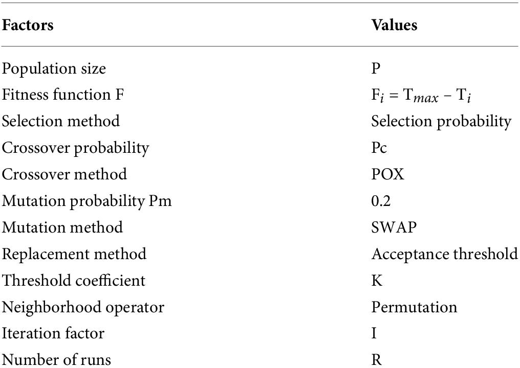
Table 2. The factors of the GATS algorithm.

Phase C and D: use the GATS algorithm to solve the FSS problem

Based on the model of the problem and the GATS algorithm, the pilot problem of small size is solved in phase C to get experience in defining the parameters of the GATS algorithm to solve the real problem of real size in phase D. Phase C and phase D will be shown in the following sections.

The pilot FSS problem

The pilot problem to be solved is a FSS problem with 10 orders, O_i, i = 1÷10. The weight W_i and the due date D_i of order i are estimated in Table 3.

TABLE 3

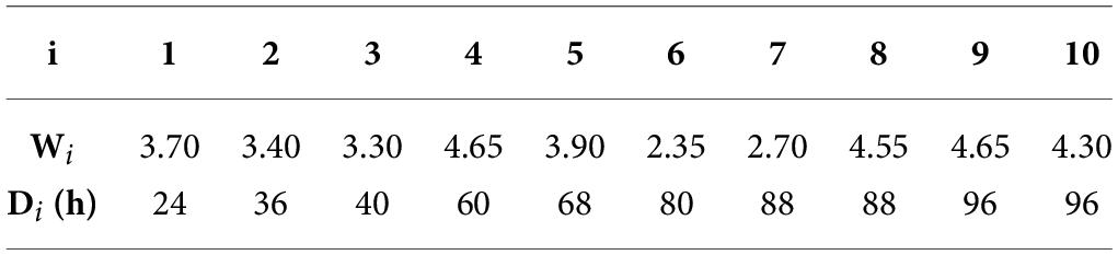
Table 3. The weight W_i, i = 1÷10 and the due date D_i, i = 1÷10 of order i.

The processing time P_ij of order i, i = 1÷10, on operation j, j = 1÷8, are estimated in Table 4.

TABLE 4

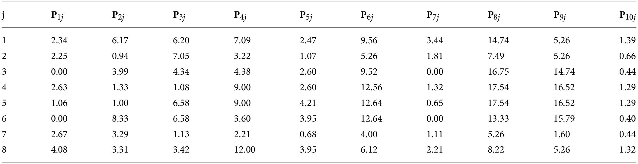
Table 4. The processing time P_ij of order i, i = 1÷10, on operation j.

The changeover times on operation j, j = 4÷8 are equal to 0.

S {}_{i j k}= 0, j = 4 \div 8 .

The changeover times in hours on operation j, j = 1÷3 are the same and depend on the current order i = 1÷10, and the next order, k = 1÷10, as shown in Table 5.

TABLE 5

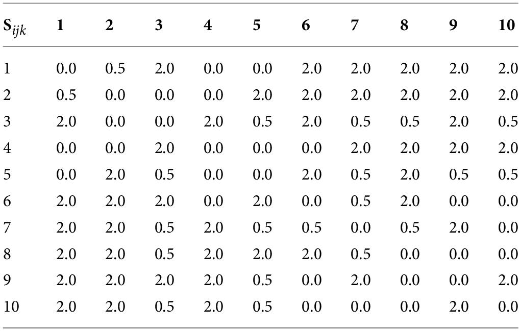
Table 5. Changeover time (h) S_ijk, j = 1÷3.

The company is currently using the EDD dispatching method. The sequence of dispatching S, the value of the objective function T are as follows.

S = (1, 2, 3, 4, 5, 6, 7, 8, 9, 10);

T = 215.95 (h)

The Gantt chart are shown in Figure 2.

FIGURE 2

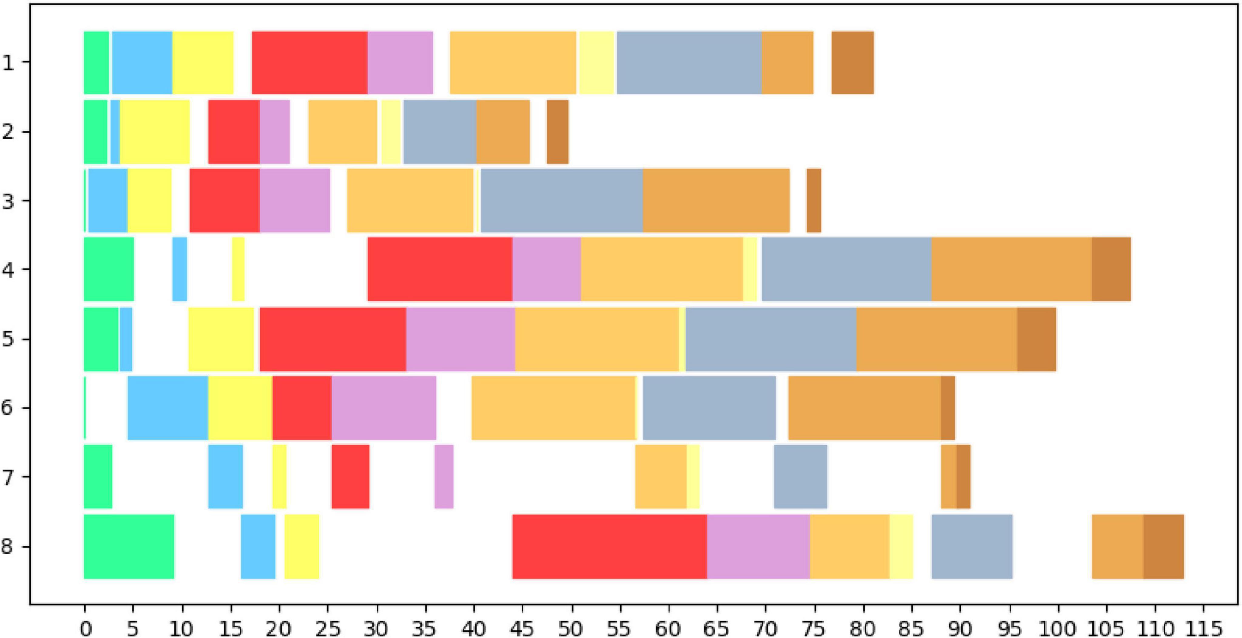
Figure 2. The Gantt chart for the pilot problem by the EDD dispatching method.

The GATS model for the pilot FSS problem

The pilot FSS problem is a NP hard problem with the size of the solution space of 10! or 3,628,800. The GATS model is used to solve the problem as follows:

Step 1: Initialize the GATS model

This step sets up factors of GATS model, including the method of coding and all factors of the algorithm. Each chromosome is a string of 10 genes. Each gene corresponds to an order. The orders are numbered from 1 to 10. The sequence of genes represents the sequence of order scheduled:

C = [G 1, G 2, G 3, G 4, G 5, G 6, G 7, G 8, G 9, G 10]

The factors of the algorithm for the pilot problem are shown in Table 6.

TABLE 6

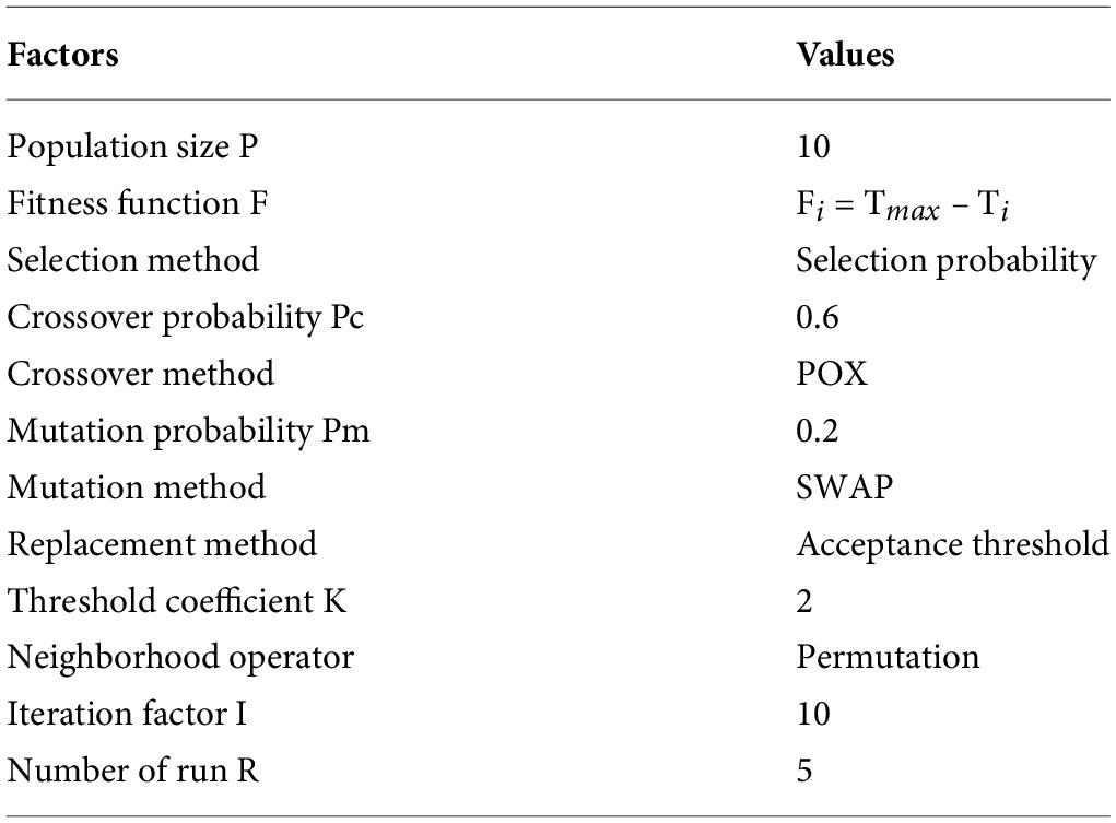
Table 6. The GATS factors for the pilot problem.

Step 2: Generate the initial population P⁽⁰⁾, set k = 0

The initial population consists of 10 chromosomes. There are three chromosomes generated from three heuristic rules: EDD, SPT, and LPT. The remaining chromosomes R1, …, R7 are randomly generated as shown in Table 7.

P {}^{(0)}= {E D D, S P T, L P T, R 1, R 2, R 3, R 4, R 5, R 6, R 7}

TABLE 7

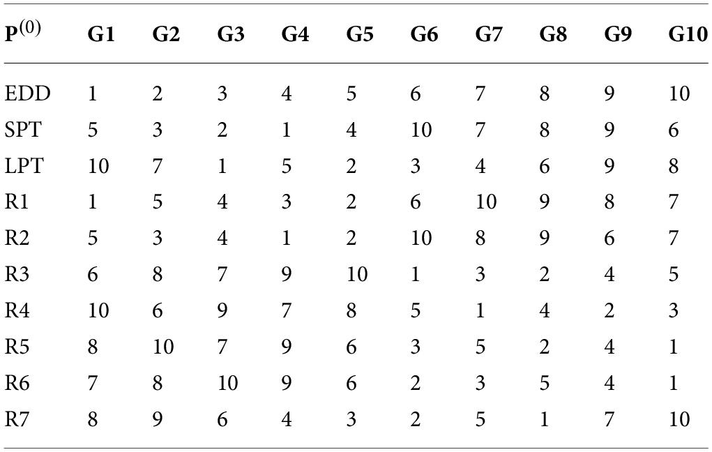
Table 7. The initial population P⁽⁰⁾.

Step 3: Generate elite population P_E⁽⁰⁾

The step uses the selection operator to generate the elite population P_E⁽⁰⁾ from P⁽⁰⁾. Each chromosome in the current population has a corresponding fitness value F_i, and is selected for inclusion in the elite population P_E⁽⁰⁾, with selection probability P_i determined as follows:

P_{i} = \frac{F_{i}}{F}, F = \sum_{i = 1}^{10} F_{i}

With population P⁽⁰⁾, the fitness values of F_i and selection probabilities P_i of chromosomes in P⁽⁰⁾ are calculated as shown in Table 8.

TABLE 8

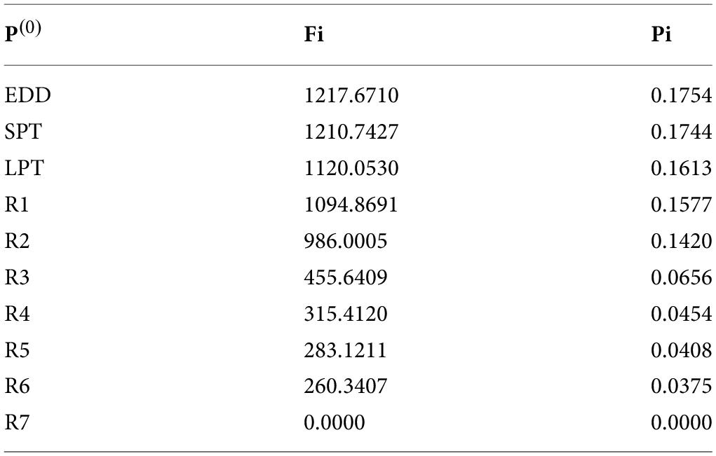
Table 8. The values of F_i and P_i.

Based on selection probabilities P_i, 10 random numbers are generated, and the chromosomes selected into the population P_E⁽⁰⁾ are as follows:

P {}_{E}^{(0)}= {R 3, R 2, L P T, S P T, E D D, S P T, S P T, E D D, R 2, R 5}

Step 4: Generate the genetic population P_G⁽⁰⁾

The genetic population P_G⁽⁰⁾ includes the new chromosome generated from the crossover and mutation operators.

The chromosomes of P_E⁽⁰⁾) are selected to be included in the crossover list P_c with the crossover probability of 0.6. After generating random numbers, the set P_c is determined as follows:

P {}_{c}= {R 3, L P T, S P T, E D D}

Each pair of chromosomes in P_c is selected to cross over by the POX method, resulting in 12 new chromosomes in population P^C with corresponding fitness values as shown in Table 9.

TABLE 9

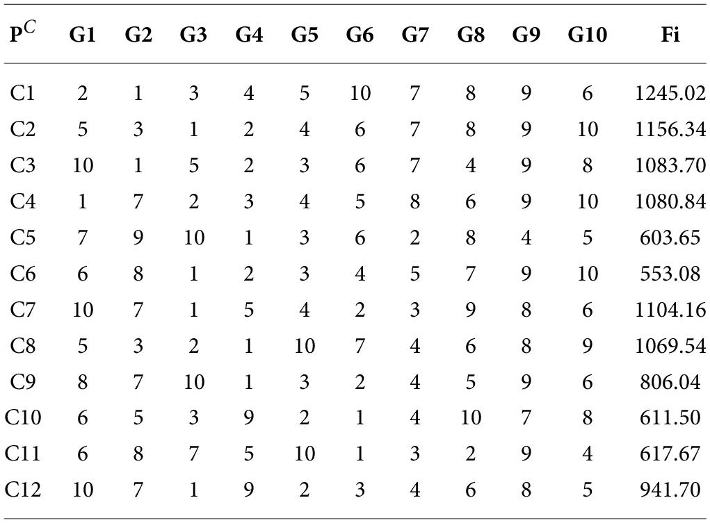
Table 9. The crossover population P^C.

The chromosomes of P_E⁽⁰⁾) are also selected to be included in the mutation list P_m with the mutation probability of 0.2. After generating random numbers, P_m is determined as follows:

P {}_{m}= {E D D}

Each chromosome in P_m is selected to mutate by the SWAP method, resulting in one new chromosome in population P^M as shown in Table 10.

TABLE 10

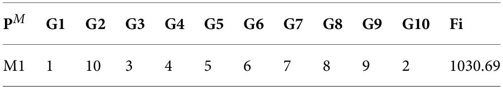
Table 10. The mutation population P^M.

After crossover and mutation, 13 new chromosomes are created in the population P_G⁽⁰⁾:

P_{G} {}^{(0)}= {C 1, C 2, C 3, C 4, C 5, C 6, C 7,

C 8, C 9, C 10, C 11, C 12, M 1}

Step 5: Generate the neighborhood population P_N⁽⁰⁾

This step uses the neighborhood operator to generate the neighborhood population P_N⁽⁰⁾ from the genetic population P_G⁽⁰⁾. Each chromosome in P_G⁽⁰⁾ will have a neighborhood defined by the neighborhood operator. In this neighborhood, the best chromosome will be selected to go forward. For example, with C1, there are nine neighboring chromosomes, of which C11 is the best and is chosen, as shown in Table 11.

TABLE 11

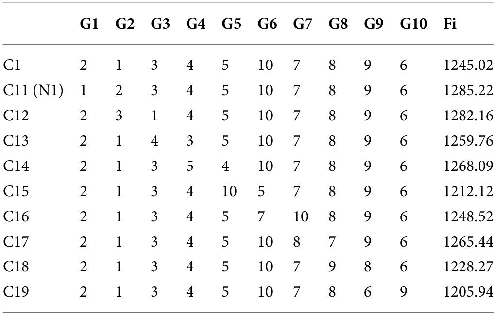
Table 11. The neighboring chromosomes of C1.

Same for the remaining chromosomes of P_G⁽⁰⁾. The neighborhood population P_N⁽⁰⁾ consists of the best neighbor chromosomes, as defined in Table 12.

P {}_{N}^{(0)}= {N 1, N 2, N 3, N 4, N 5, N 6, N 7, N 8, N 9,

N 10, N 11, N 12, N 13}

TABLE 12

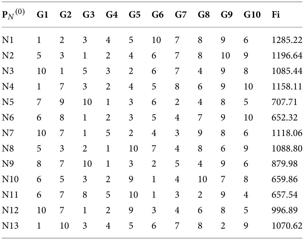
Table 12. The neighborhood population P_N⁽⁰⁾.

Step 6. Generate the next population P⁽¹⁾

This step uses the replacement operator to generate the next population P⁽¹⁾ from the populations P_G⁽⁰⁾ and P_N⁽⁰⁾. The chromosomes from P_G⁽⁰⁾ and P_N⁽⁰⁾ will be added to the current population P⁽⁰⁾ to make the next population P⁽¹⁾, if their fitness values exceed the acceptable threshold. With the threshold coefficient K of 2 and the population size P of 10, the acceptable threshold is the fitness value of the 5th chromosome of P⁽⁰⁾ in the ranking.

To keep the next population size constant, the chromosomes with the lowest value are removed from the next population. After applying the replacement operator, the next population P⁽¹⁾ is determined as in Table 13.

P {}^{(1)}= {N 1, C 1, E D D, S P T, N 2, N 4, C 2, L P T, N 7, C 7}

TABLE 13

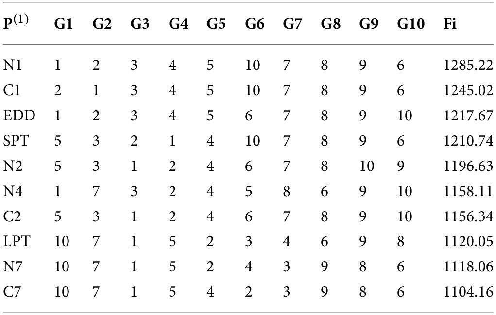
Table 13. The next population P⁽¹⁾.

Step 7. Check the termination rule

After iteration 1, N1 is the best chromosome with the best fitness value of 1285.22 and the best objective value of 148.40, appearing only once. The termination rule is not satisfied, so iteration 2 is executed. The results after 14 iterations are shown in Table 14.

TABLE 14

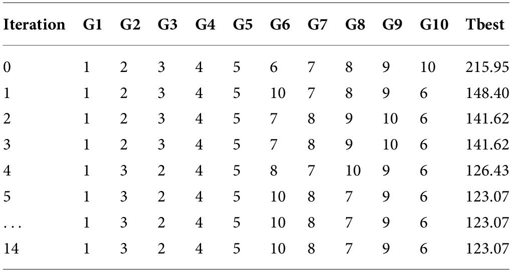
Table 14. The results after 14 iterations.

Seeing that from the 5th iteration to the 14th iteration, the best objective value remains the same, the termination rule is satisfied, and the run ends. The scheduling result in this run is as follows:

S = (1, 3, 2, 4, 5, 7, 8, 9, 10, 6),

T b e s t = 123.07 (h)

Step 8. Run the algorithm for five times to choose the best scheduling result

The algorithm is run five times with the results as shown in Table 15.

TABLE 15

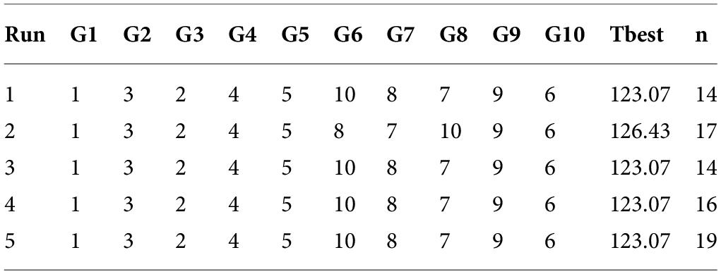
Table 15. The results after four runs.

The best scheduling result is found on the 1st run, with a number of iterations n of 14. The sequence of dispatching S, the value of the objective function, and the Gantt chart are as follows:

S = (1, 3, 2, 4, 5, 7, 8, 9, 10, 6);

T b e s t = 123.07 (h)

Comparing to the currently used dispatching method, EDD, the value of the objective function T has been improved, reduced from 215.95 (h) to 123.07 (h).

The GATS model for the real FSS problem

The real problem to be solved is a FSS problem with 120 orders, scheduling on four machines. Each order has three parts, P1, P2, and P3, processed in eight operations, distributed on the four machines as in Figure 1. Problem data has been collected to estimate the parameters of the weight W_i, the due date D_i of order i, i = 1÷120, the processing time P_ij of order i, i = 1÷120, on operation j, j = 1÷8, and of the changeover times S_ijk, i = 1÷120, j = 1÷8, k = 1÷120.

The company is currently using the EDD dispatching method. The total weighted tardiness time T and the number of late delivery orders N of the real size problem are as follows:

T = 354.95 (h),

N = 31 .

The above GATS model has been coded on the Python platform and applied to solve the real problem. The real problem size is larger than the pilot problem size, so some factors of the GATS model have been changed to suit the real problem. The parameters or factors of the GATS model for the real problem are as in Table 16.

TABLE 16

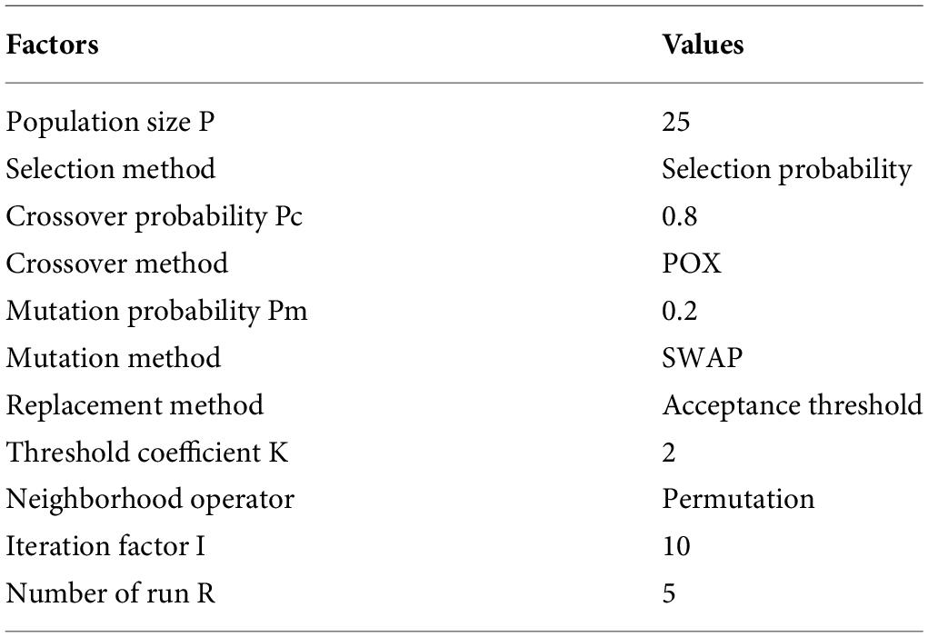
Table 16. The GATS factors for the real problem.

The sequence of the order to be scheduled by the GATS model is as follows: [1, 2, 3, 103, 5, 119, 6, 69, 8, 9, 11, 14, 12, 15, 13, 16, 17, 76, 18, 78, 21, 22, 24, 101, 25, 27, 10, 90, 28, 29, 31, 30, 33, 35, 32, 34, 37, 36, 38, 44, 39, 40, 41, 42, 19, 45, 47, 46, 49, 48, 52, 54, 51, 53, 55, 56, 57, 59, 91, 60, 61, 62, 63, 65, 64, 66, 7, 67, 68, 70, 85, 73, 75, 72, 77, 74, 43, 83, 79, 20, 81, 84, 82, 71, 87, 88, 89, 86, 26, 92, 58, 94, 95, 93, 96, 98, 99, 97, 100, 23, 102, 4, 105, 104, 106, 107, 108, 109, 111, 110, 50, 112, 80, 117, 116, 115, 114, 113, 118, 120]. The Gantt chart is shown in Figure 3.

FIGURE 3

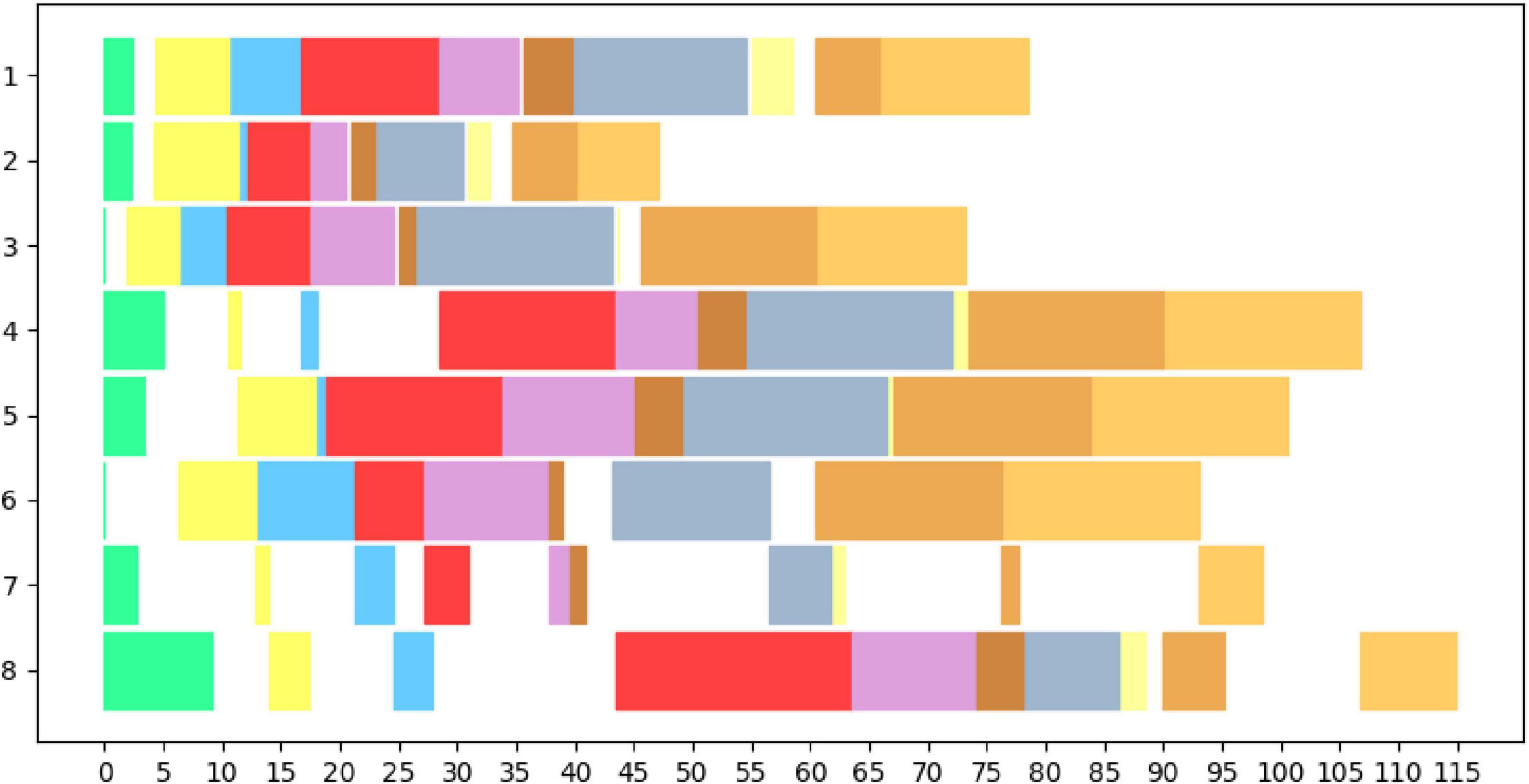
Figure 3. The Gantt chart by the GATS model.

The total weighted tardiness time T and the number of late delivery orders N of the real size problem is as follows:

T = 277.50 (h),

N = 5 .

The total weighted tardiness time T has been decreased by 21% from 354.95 (h) to 277.50 (h). The number of late delivery orders N has been decreased from 31 to 5.

Conclusion

The FSS problem to be solved is modeled with the objective to minimize the total weighted tardiness of orders, and constraints on the sequence of orders, on the sequence of operations in the orders, and on machine changeover time.

The GATS algorithm is developed. In the algorithm, GA is used as the platform for global search, and TS is used to support GA in local search. GA diversifies the search by exploring the search space, and TS intensifies the search by exploiting the best solutions found. GA generates the elite population and generates genetic populations from the elite population by using GA operators. Then TS generates the neighborhood population from the genetic population by using neighborhood operators. Finally, GA generates the next population from the current population, the elite population, and the neighborhood population by using replacement operators.

Based on the model of the problem, the GATS algorithm is used to solve the pilot problem of small size, with 10 orders, scheduling on four machines. The total weighted tardiness time according to the algorithm (123.07 h) is better than the total weighted tardiness time according to the EDD heuristic currently used (215.95 h).

The algorithm is also used to solve the real FSS problem with 120 jobs on four machines. The results show that the algorithm gives better results than the current heuristic EDD method. The total weighted tardiness time T has been decreased by 21% from 354.95 (h) to 277.50 (h). The number of late delivery orders N has been decreased from 31 to 5.

However, the factors of the model, including the population size P, the crossover probability P_c, the mutation probability P_m, the method of crossover, of mutation, the method of finding the neighborhood chromosomes, the method and parameter of the termination rule, etc., are only selected empirically, so the results are not very good. Future research is to use experimental design DOE to optimize the model factors to get suboptimal results.

Funding

The authors declare that no financial support was received for the research, authorship, and/or publication of this article.

Conflict of interest

The authors declare that the research was conducted in the absence of any commercial or financial relationships that could be construed as a potential conflict of interest.

References

1. Etiler O, Toklu B, Atak M, Wilson J. A genetic algorithm for flow shop scheduling problems. J Oper Res Soc. (2004) 55:830–5. doi: 10.1057/palgrave.jors.2601766

CrossRef Full Text | Google Scholar

2. Engin O, Ceran G, Yilmaz MK. An efficient genetic algorithm for hybrid flow shop scheduling with multiprocessor task problems. Appl Soft Comp. (2011) 11:3056–65. doi: 10.1016/j.asoc.2010.12.006

CrossRef Full Text | Google Scholar

3. Phong NN, Ngan K, Thi N, Huyen T, Thi TV. Application of genetic algorithm, GA to solve a flow shop scheduling problem with changeover times in operations: a case study. BOHR Int J Oper Manag Res Pract. (2024) 3(1):19–26. doi: 10.54646/bijomrp.2024.24

CrossRef Full Text | Google Scholar

4. Pezzella F, Morganti G, Ciaschetti G. A genetic algorithm for the Flexible Job-shop Scheduling Problem. Comp Oper. Res. (2007) 35:3202–12.

Google Scholar

5. Gupta J, Palanimuthu N, Chen C-L. Designing a tabu search algorithm for the two-stage flow shop problem with secondary criterion. Prod Plann Cont Manage Oper. (1999) 10:251–65. doi: 10.1080/095372899233217

CrossRef Full Text | Google Scholar

6. Phong NN, Nhi T, Thi N. Application of Tabu Search, TS to solve a flow shop scheduling problem with changeover times in operations. A case study. BOHR Int J Oper Manag Res Pract. (2024) 3(1):1–7. doi: 10.54646/bijomrp.2024.22

CrossRef Full Text | Google Scholar

7. Burduk A, Musiał K, Kochanska J, Górnicka D, Stetsenko A. Tabu search and genetic algorithm for production process scheduling problem. Sci J Logist. (2019):181–9. doi: 10.17270/J.LOG.2019.315

CrossRef Full Text | Google Scholar

8. Umam MS, Mustafid M, Suryono S. A hybrid genetic algorithm and tabu search for minimizing makespan in flow shop scheduling problem. J King Saud Univ. Comp Inform Sci. (2022) 34:7459–67. doi: 10.1016/j.jksuci.2021.08.025

CrossRef Full Text | Google Scholar

9. Ben-Daya M, Al-Fawzan M. A tabu search approach for the flow shop scheduling problem. Eur J Oper Res. (1997) 09:88–95.

Google Scholar

10. Phong NN, Ngan K, Thi N. Application of GATS, a hybrid mega heuristic model, to solve flow shop scheduling problems FFS with changeover times in operations. A case study. The 4th International Conference on Applied Convergence Engineering (ICACE 2023). Ho Chi Minh City, Vietnam: Ho Chi Minh City University of Technology, VNU-HCM (2023).

Google Scholar

11. Phong NN, Nhi T, Thi N. Application of TSGA, a hybrid mega heuristic model, to solve flow shop scheduling problems FFS with changeover times in operations. A case study. The 4th International Conference on Applied Convergence Engineering (ICACE 2023). Ho Chi Minh City, Vietnam: Ho Chi Minh City University of Technology, VNU-HCM (2023).

Google Scholar

12. Phong NN, Trang T, Le N. Application of GATS, a hybrid mega heuristic model, and DOE, Design of Experiment, to solve flexible flow shop scheduling problems - A case study. BOHR Int J Oper Manag Res Pract. (2023) 2(1):28–35. doi: 10.54646/bijomrp.2023.14

CrossRef Full Text | Google Scholar

© The Author(s). 2026 Open Access This article is distributed under the terms of the Creative Commons Attribution 4.0 International License (https://creativecommons.org/licenses/by/4.0/), which permits unrestricted use, distribution, and reproduction in any medium, provided you give appropriate credit to the original author(s) and the source, provide a link to the Creative Commons license, and indicate if changes were made.

Application of GATS, a hybrid meta-heuristic model of genetic algorithm and tabu search, to solve a real-size problem of flow-shop scheduling with changeover times in operations: A case study in the flushing-kit-manufacturing industry

Introduction

Literature review

Research methodology

Phase A: construct the model of the FSS problem

Phase B: construct the GATS algorithm

Step 1: Initialize the GATS model

Step 2: Generate the initial population P(0). Set k = 0

Step 3: Generate elite population PE(k)

Step 4: Generate the genetic population PG(k)

Step 5: Generate the neighborhood population PN(k)

Step 6: Generate the next population P(k+1). Set k = k+1

Step 7: Check the termination rule

Step 8: Run the algorithm a number of times to choose the best scheduling result

Phase C and D: use the GATS algorithm to solve the FSS problem

The pilot FSS problem

The GATS model for the pilot FSS problem

Step 1: Initialize the GATS model

Step 2: Generate the initial population P(0), set k = 0

Step 3: Generate elite population PE(0)

Step 4: Generate the genetic population PG(0)

Step 5: Generate the neighborhood population PN(0)

Step 6. Generate the next population P(1)

Step 7. Check the termination rule

Step 8. Run the algorithm for five times to choose the best scheduling result

The GATS model for the real FSS problem

Conclusion

Funding

Conflict of interest

References

Step 2: Generate the initial population P⁽⁰⁾. Set k = 0

Step 3: Generate elite population P_E^(k)

Step 4: Generate the genetic population P_G^(k)

Step 5: Generate the neighborhood population P_N^(k)

Step 6: Generate the next population P^(k+1). Set k = k+1

Step 2: Generate the initial population P⁽⁰⁾, set k = 0

Step 3: Generate elite population P_E⁽⁰⁾

Step 4: Generate the genetic population P_G⁽⁰⁾

Step 5: Generate the neighborhood population P_N⁽⁰⁾

Step 6. Generate the next population P⁽¹⁾