Bohr article

Introduction

Effective inventory management is crucial for the smooth operation of businesses, as it ensures optimal stock levels while minimizing costs. In the context of an equipment processing company in Vietnam, efficient inventory control holds significant importance. Currently, the company relies on an experiential inventory model for ordering, which lacks consideration for demand forecasting and cost-related factors.

However, the study has recognized some problems with this model, which are: the inappropriate planning model leads to the situation of excessive inventory, which increases inventory costs; the cost of raw materials is increasing, and continuing with the current lot sizing planning of the company will result in higher inventory costs and a shortfall in purchasing budget; the warehouse space for materials is limited, and ineffective inventory control can lead to warehouse overload.

A model is proposed to address this problem. An inventory system is developed for multiple materials with discrete, known demand, with storage, budget, and order quantity constraints, with an All Unit Discount (AUD) for each item.

The model determines the optimal order quantity of products to minimize the total inventory cost during the planning period. Real-life situations increase the complexity of the model; the Genetic Algorithm (GA) algorithm is used to solve the proposed mathematical model.

The GA is an optimization method inspired by natural selection, capable of finding optimal or near-optimal solutions by evolving a population of potential solutions through selection, crossover, and mutation. It is widely used for solving complex problems in various fields.

Design of experiments (DOEs) is used to optimize the parameters of the GA model. The results of the heuristic methods being used, of the GA, and of the GA with DOE are compared to evaluate their effectiveness.

Literature review & research methodology

Literature review

Inventory dynamic lot-sizing

The stochastic inventory models first appeared in the literature in the early 1950s in specialized papers by Arrow et al. (1) and Dworetzky et al. (2, 3). These models were developed to capture the uncertainty and variability that exist in most real-world inventory situations but are often assumed away in deterministic inventory models. Due to the combination of uncertainty in demand and/or lead time, the fundamental mathematical structure for stochastic inventory models is more complex than that for deterministic models and requires management to have policy statements regarding system inventory performance measures, such as service level or fill rate.

Inventory models can be classified into two main categories by Aggarwal (4): static and dynamic models. In a static model, the parameters remain constant over time, such as constant demand rate, constant lead time, and fixed costs. On the other hand, dynamic models involve parameters that continuously change over time, such as varying demand rates, delivery lead times, and cost factors that affect total inventory costs. Dynamic models typically require more complex and challenging calculations compared to static models.

Lot sizing models can be classified into static and dynamic models. Static models, such as the Economic Order Quantity (EOQ) model, plan lot sizes with constant demand and inventory costs. Dynamic models plan lot sizes with variable demand and inventory costs.

Genetic algorithm

Genetic Algorithm (GA) is a meta-heuristic algorithm that starts with a population of potential solutions represented as chromosomes. Through selection, crossover, and mutation operators, the algorithm evolves the population over many generations. This process continues until a stopping condition is reached. GAs are effective in exploring large search spaces and finding near-optimal solutions for complex problems. GAs are used in a wide variety of fields and are known for their adaptability and flexibility.

Notably, GA has been utilized in previous research studies to address specific inventory-related challenges. For instance, Mondal et al. (5) developed a multi-item fuzzy EOQ model, and Maiti et al. (6) investigated the optimization of imperfect production processes for damageable items. Both studies successfully employed GA to solve their respective mathematical models. The versatility and effectiveness of GA make it a valuable tool in addressing complex inventory management problems and optimizing decision-making processes.

Research methodology

The research methodology includes the following steps.

1. Developing the mathematical model of the dynamic lot-sizing (DLS) problem.

2. Developing the GA algorithm to solve the DLS problem.

3. Applying the GA algorithm to solve the DLS problem.

4. Using DOE to optimize the parameters of the GA model.

5. Applying the GA algorithm with optimized parameters to solve the DLS problem.

Mathematical model of the dynamic lot-sizing problem

Consider a company that plans inventories for several materials with known demand that varies in cycles over a finite planning horizon of N periods. The initial inventory level for all items is zero, and only one order is placed for a particular item in each cycle.

Additionally, there are limitations on the order quantity of each item, and ordered quantities are delivered in batch sizes without the possibility of splitting batches. The company also has restrictions on shortages, storage space, and the available budget. Quantity discount policies are implemented based on the prevailing circumstances. The objective is to determine the optimal order quantities for the products, variable demand in each period, to minimize the total cost of the inventory system while satisfying the given constraints. The problem to be solved is a DL problem with three items, i = 1 ÷ 3, with 12 periods, j = 1 ÷ 12.

Assumptions

1. The initial inventory level for the first cycle of all items is 0.

2. The price level is known and can vary depending on the order quantity.

3. There are fixed and unchanged unit costs, and there is no price inflation.

Parameters

Item index i: i = 1, 2, 3

Period index j: j = 1÷12

Breakpoint index k: k = 1, 2, 3

TC: total inventory cost (USD)

TO: total purchasing cost (USD)

TH: total holding cost (USD)

TP: total ordering cost (USD)

O_i: ordering cost per order time of item i in period j (USD/one order)

X_i,_j: initial inventory level of item i in period j (in j = 1 the initial inventory of all items is zero)

D_i,_j: demand of item i at period j (unit)

T_j: total time elapsed up to period j

I_i: inventory level of item i at time t (T_j < t <T_j+1)

H_i: inventory holding cost per unit of item i during a period (USD/unit/year)

q_i,_k: the kth discount breakpoint of ith product (q_i,1 = 0)

P_i,_k: The purchase price of item i at breakpoint k under the AUD policy

S: total available storage space (m²)

s_i: required warehouse space per unit of ith product (m²/unit)

C: total available budget ($)

M₁: an upper bound for Q_i,_j.

Decision variables

Q_i,_j: ordering quantity of item i in period j.

W_i,_j: a binary decision variable; determining whether there is an order placement in a period; set equal one if a purchase of an item i is made in period j, and zero otherwise.

U_i,_j,_k: a binary decision variable; determine if there is an order placement at price point k; set equal one if item i is purchased at price breakpoint k in period j, and zero otherwise.

Objective function

The beginning inventory of item i:

X_{i j + 1} = X_{i, j} + Q_{i, j} - D_{i, j} (1)

The total ordering cost:

T O = \sum_{i = 1}^{m} \sum_{j = 1}^{N - 1} O_{i} W_{i j} (2)

In order to obtain the total holding cost, we first calculate I_i(t) for (T_j < t < T_j+1):

I_{i} (t) = (X_{i, j} + Q_{i, j}) - \frac{D_{i, j} (t - T_{j})}{T_{j + 1} - T_{j}} (3)

Therefore, the holding cost of item i in the interval [T_j, T_j ₊ ₁] is

T H = H_{i} \int_{T_{T_{J}}}^{j + 1} I_{i} (t) d t (4)

Inserting Equations (3) in (4):

T H = \sum_{i = 1}^{m} \sum_{j = 1}^{N} H_{i} (T_{j + 1} - T_{j}) [X_{i j} Q_{i j}

+ \frac{D_{i j} T_{j}}{T_{j + 1} - T_{j}} - \frac{D_{i j} (T_{j + 1} + T_{j})}{2 (T_{j + 1} - T_{j})} (5)

The purchasing cost corresponded to AUD policies obtained as follows:

{\begin{matrix} \begin{matrix} P_{i, 1}; 0 < Q_{i j} \leq q_{i, 2} \\ P_{i, 2}; q_{i, 2} < Q_{i j} \leq q_{i, 3} \\ ⋮ \end{matrix} \\ P_{i, K}; q_{i, K} < Q_{i j} \end{matrix}

The purchasing cost under the AUD scheme:

TP = \sum_{i = 1}^{m} \sum_{j = 1}^{N - 1} \sum_{k = 1}^{K} P_{i, k} Q_{i j} U_{i j, k} (6)

The total cost of the inventory control problem includes total ordering cost, total holding cost, and total purchasing cost:

TC = TO + TH + TP (7)

From Equations (2), (5), (6), and (7), the objective function is as follows.

M i n T C = \sum_{i = 1}^{m} \sum_{j = 1}^{N - 1} O_{i} W_{i j} + \sum_{i = 1}^{m} \sum_{j = 1}^{N} H_{i} (T_{j + 1} - T_{j})

[X_{i j} + Q_{i j} + \frac{D_{i j} T_{j}}{T_{j + 1} - T_{j}} - \frac{D_{i j} (T_{j + 1} + T_{j})}{2 (T_{j + 1} - T_{j})}

+ \sum_{i = 1}^{m} \sum_{j = 1}^{N - 1} \sum_{k = 1}^{K} P_{i, k} Q_{i j} U_{i j, k}

Constraints

X_{i, 1} = 0, i = 1 \div M

\sum_{i = 1}^{m} (X_{i j} + Q_{i j}) s_{i} \leq S; j = 1 \div N

\sum_{i = 1}^{m} Q_{i j} P_{i} \leq C; j = 1 \div N

Q_{i, j} \geq M_{i}; i = 1 \div m & j = 1 \div N

\sum_{k = 1}^{K} U_{i, j, k} = 1; i = 1, \div m & j = 1 \div N

X_{i j} \geq 0; i = 1 \div m & j = 1 \div N

Q_{i j} \geq 0 \forall i, j

W_{i j} \in {0, 1} \forall i, j

U_{i, j, k} \in {0, 1} \forall i, j, k

B_{i} V_{i} \in N^{*}

Constraint 1 presents the initial inventory of all items is zero. Constraint 2 is related the area of the storage that was enough to store the ordered items. Constraint 3 is the allowed budget for the order. Constraint 4 presents an upper bound for Q_i,_j_. Constraint 5 represents that there must be an order. Constraint 6 ensures the positive inventory levels. The remaining constraints help tighten the model.

The company is currently planning based on experience. The current objective value is as follows.

T C = 25, 182 .

The GA model for solving the dynamic lot-sizing problem

The above DL problem is a non-linear problem with a solution space of 11^12×3,or11³⁶. The GA model is used to solve the problem.

The method of coding

Within this study, the chromosomes employed are represented as matrix, denoting the order quantities of items (r_i,_j) during each respective period. To provide a visual illustration, Figure 1 portrays the chromosome structure for a scenario comprising four products and four periods. In this depiction, the rows and columns correspond to the number of items and periods, respectively.

FIGURE 1

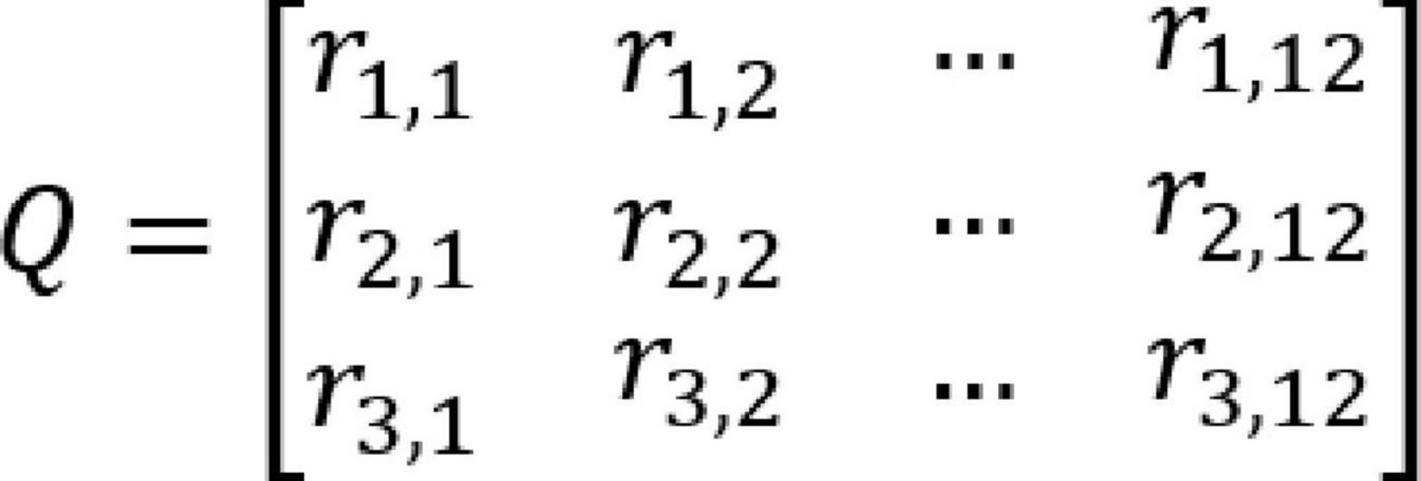
Figure 1. The structure of a chromosome.

The GA procedure

The GA parameters are shown in Table 1 as follows.

TABLE 1

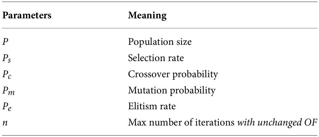
Table 1. The Genetic Algorithm (GA) parameters.

The GA factors are shown in Table 2 as follows.

TABLE 2

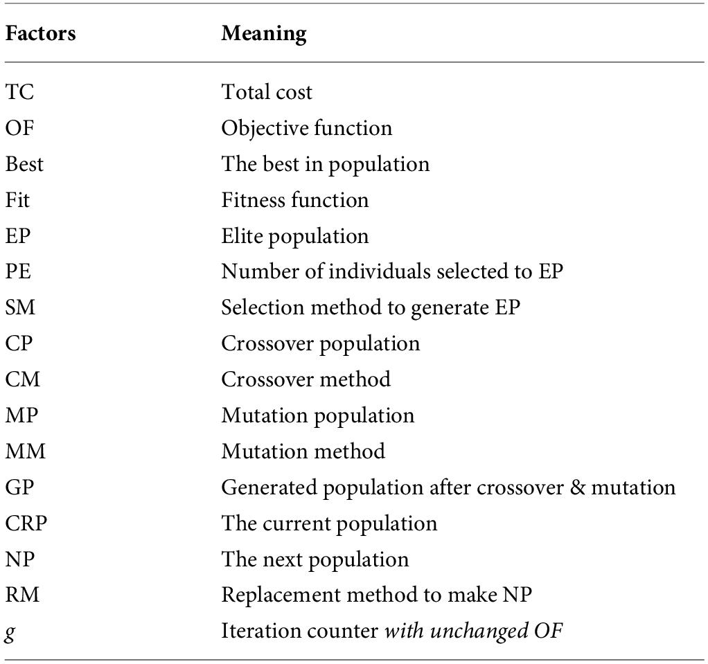
Table 2. The GA factors.

The GA pseudo code is as follows.

Begin

Set parameters (P, P_s, P_c, P_m, P_e, n)

Randomly initialize population P

OF = TC(P)

Best₀ = min OF

Fit = 1/OF²

g = 0

While (g < n)

Select individuals from CRP to EP (Using SM with selection probability P_s)

Crossover (Using CM, chromosomes in EP chosen to CP if random [0,1] < P_c)

Mutation (Using MM, chromosomes in EP chosen to MP if random [0,1] < P_m)

Calculate the objective function for new individuals GP

Select individuals from GP to NP (Using RM with elitism probability P_e)

Update values (CRT;Best)

IfBest_{i + 1}−Best_i≥0, Theng = g + 1, Elseg = 0

EndWhile

Return CRP; Best

End

The steps involved in the proposed GA algorithm are as follows.

Step 1. Establish the GA parameters.

Step 2. Initialize the population randomly, consisting of P individuals.

Step 3. Evaluate the objective function to quantify the fitness of each individual within the population.

Step 4. Select individuals for the EP from CRP by using SM with selection probability P_s.

Step 5. Apply the crossover operator to each pair of chromosomes, guided by the CM & P_c.

Step 6. Implement the mutation operation on each chromosome, guided by the MM & P_m.

Step 7. Generate the GP, including offspring generated through crossover and mutation.

Step 8. Generate the next population NP by replacing bad chromosomes in CRP with chromosomes in GP by using RM with elitism probability P_e.

Step 9. Check if the stopping criterion has been met. If the criterion is satisfied, terminate the algorithm. If not, proceed to Step 3 to continue the iterative process.

Applying the GA model for solving the DLS problem

The GA parameters & factors

In order to solve the DLS problem, the GA parameters are chosen in Table 3 as follows.

TABLE 3

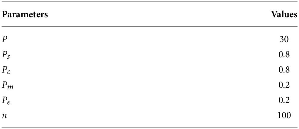
Table 3. The GA parameters and factors.

The GA factors are chosen in Table 4 as follows.

TABLE 4

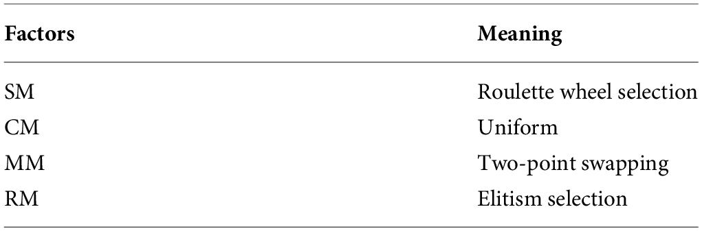
Table 4. The GA factors.

The GA operators

The selection operator

The selection operator selects chromosomes from the CRP to EP by using the Roulette Wheel Selection method with selection probability P_s as presented in reference (7).

The crossover operator

Pasandideh et al. (8) also proposed a commonly used crossover operator called the uniform crossover. To perform the crossover operation, firstly, a binary chromosome is randomly generated. Then, within the generated binary chromosome, the genes with a value of one are considered. The genes of the parents are crossed over in such a way that they have the same positions with a value of one. An example is shown in Figure 2.

FIGURE 2

Figure 2. An example of the crossover operator.

The mutation operator

The two-point swapping mutation operator, as mentioned by Tsai in (9), is applied by randomly selecting two points on the chromosome and exchanging their positions with each other. An example is shown in Figure 3.

FIGURE 3

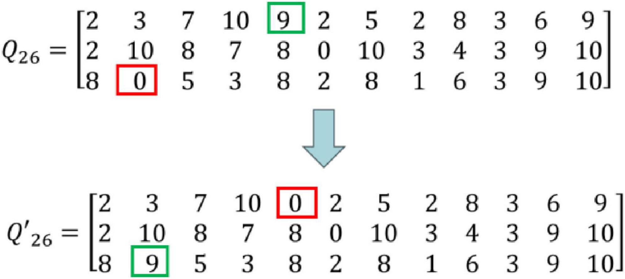
Figure 3. An example of the mutation operation.

The replacing operator

Using the elitism selection method, the top P_e×P best individuals are preserved, which in this case would be 0.2 × 30 = 5 best individuals from the previous population, without undergoing crossover and mutation. Then, the remaining 25 chromosomes are selected for the next generation using the roulette wheel selection method.

The stopping criterion

After n consecutive iterations without any improvement, the model end. And the final result of TC is shown in the graph below in Figure 4.

FIGURE 4

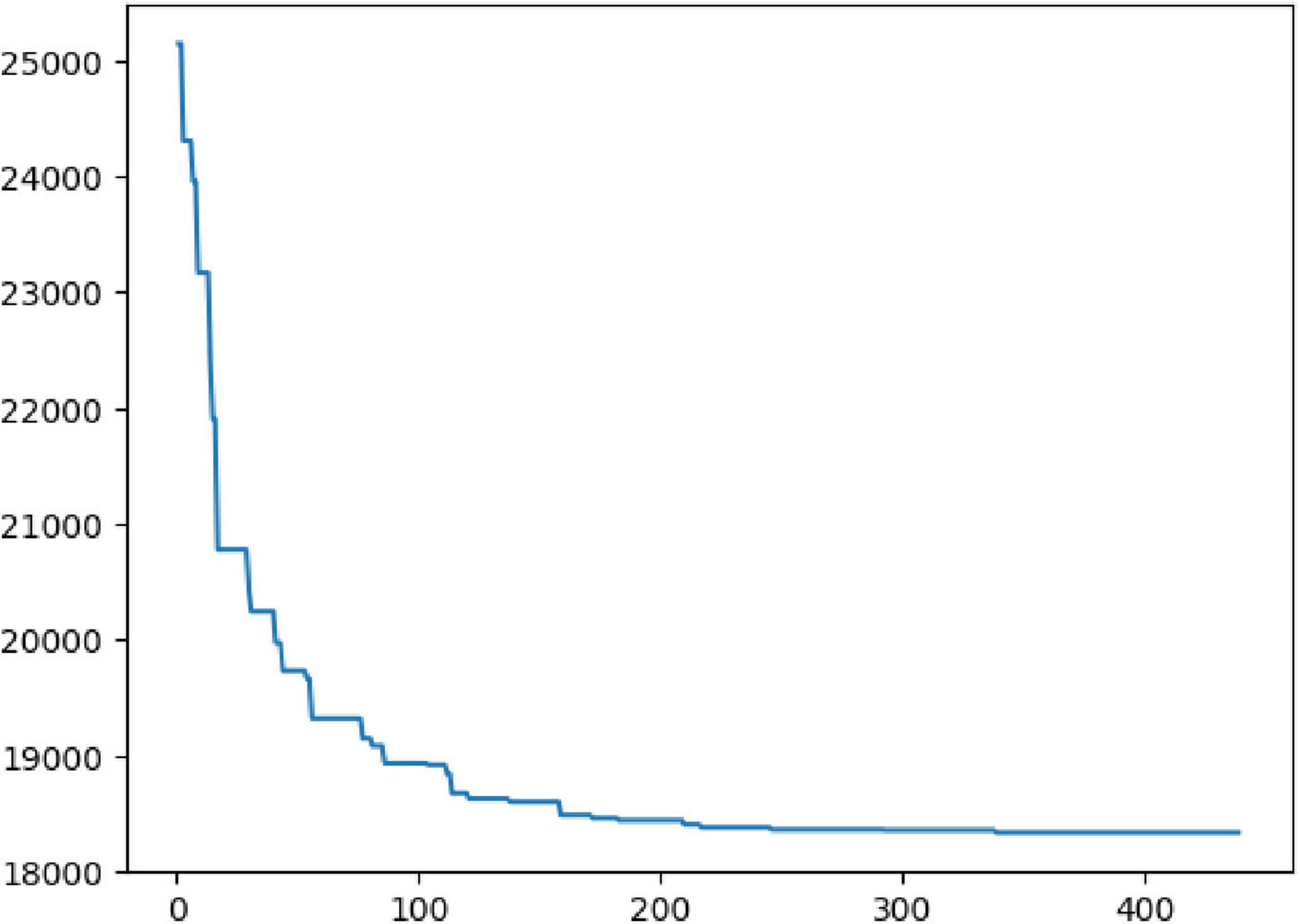
Figure 4. The result of the objective function of the GA model.

The algorithm’s results regarding the optimal batch size and the objective function of inventory cost are as follows.

Q = [\begin{matrix} 7 & 2 & 0 & 0 & 9 & 0 & 0 & 1 & 2 & 5 & 0 & 2 \\ 7 & 3 & 4 & 0 & 3 & 6 & 7 & 9 & 9 & 0 & 1 & 7 \\ 4 & 7 & 6 & 0 & 6 & 0 & 4 & 0 & 1 & 4 & 0 & 4 \end{matrix}]

TC = 18, 336.725

Applying the GA with DOE to solve the DLS problem

The parameters of the above GA model were selected empirically, resulting in suboptimal results. To optimize the model parameters, an experimental design approach is employed.

The 2^k experiment

Initially, a 2^k experiment is conducted with the input factors P, n, P_s, P_c, P_m, and P_e, and the output factor TC, representing the total inventory cost. The levels of the input factors are chosen as follows in Table 5.

TABLE 5

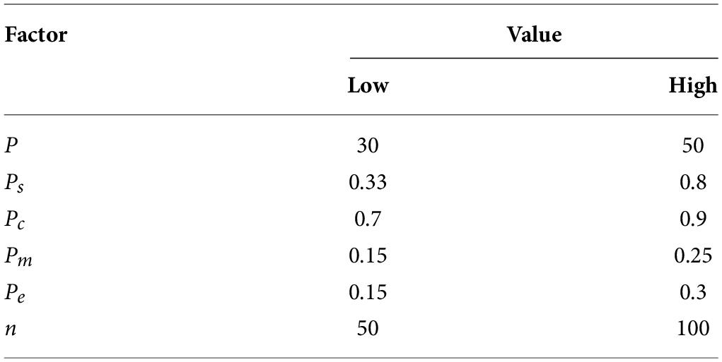
Table 5. Two levels of the input factors.

With the sample size of 3, the total number of experiments is 36. After the experiment, the ANOVA table is shown in Figure 5.

FIGURE 5

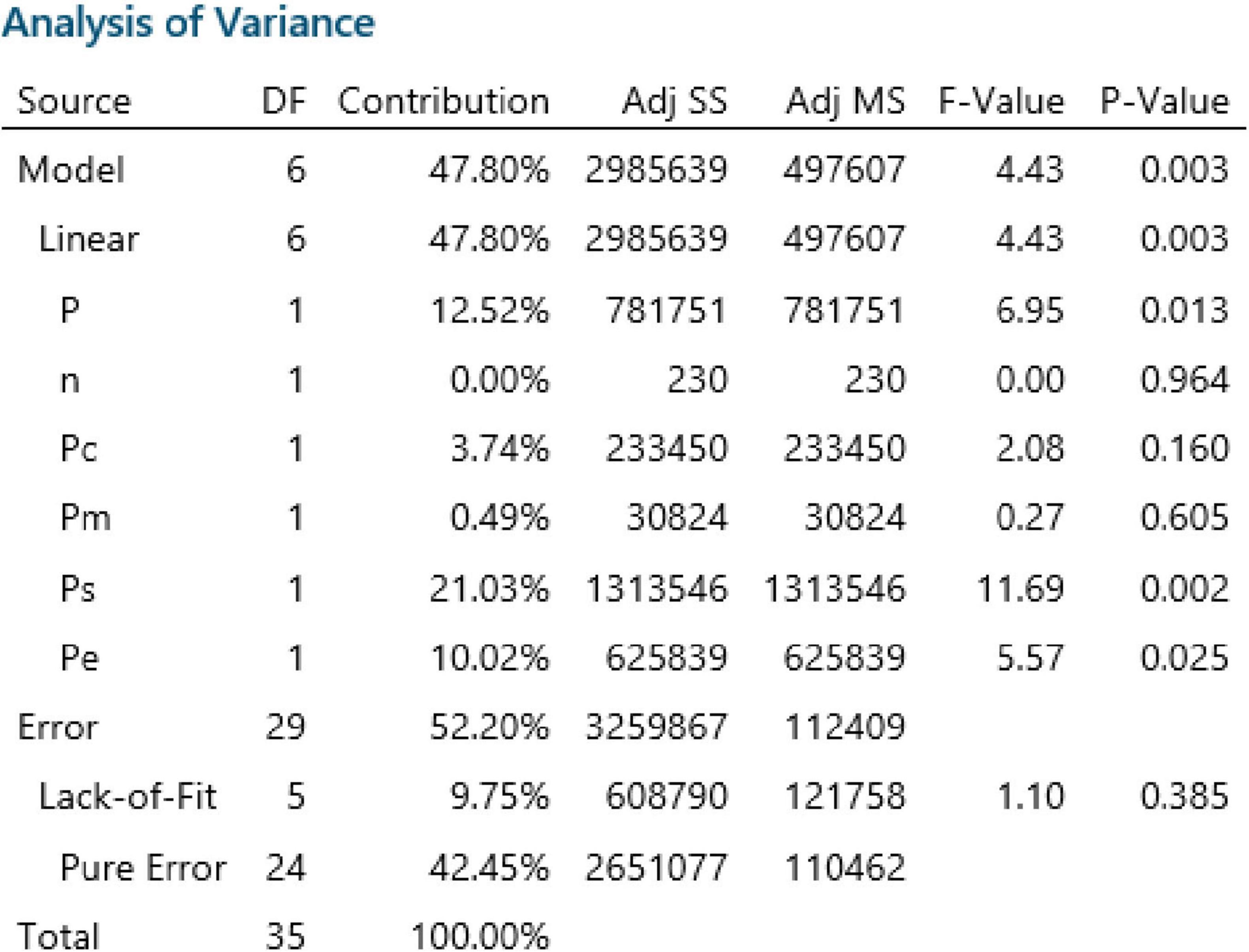
Figure 5. Analysis of variance of the experiment.

From the above ANOVA table, with α of 0.05, the affected factors are factors P, P_s, and P_e. The following Figure 6 Pareto chart illustrates the level of influence of factors from high to low.

FIGURE 6

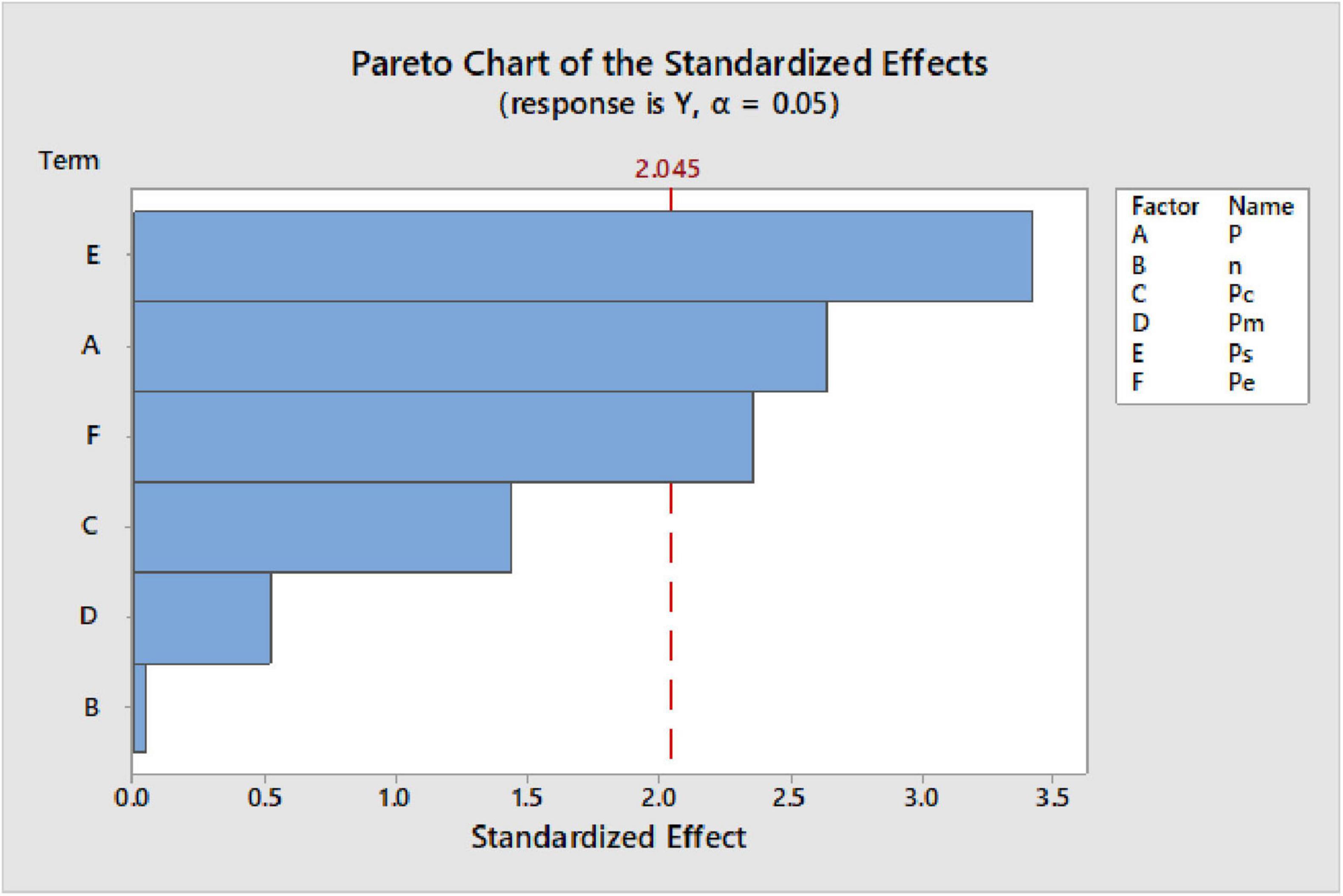
Figure 6. The Pareto chart illustrates the level of influence of factors from high to low.

The optimized values of parameters are shown in Figure 7.

FIGURE 7

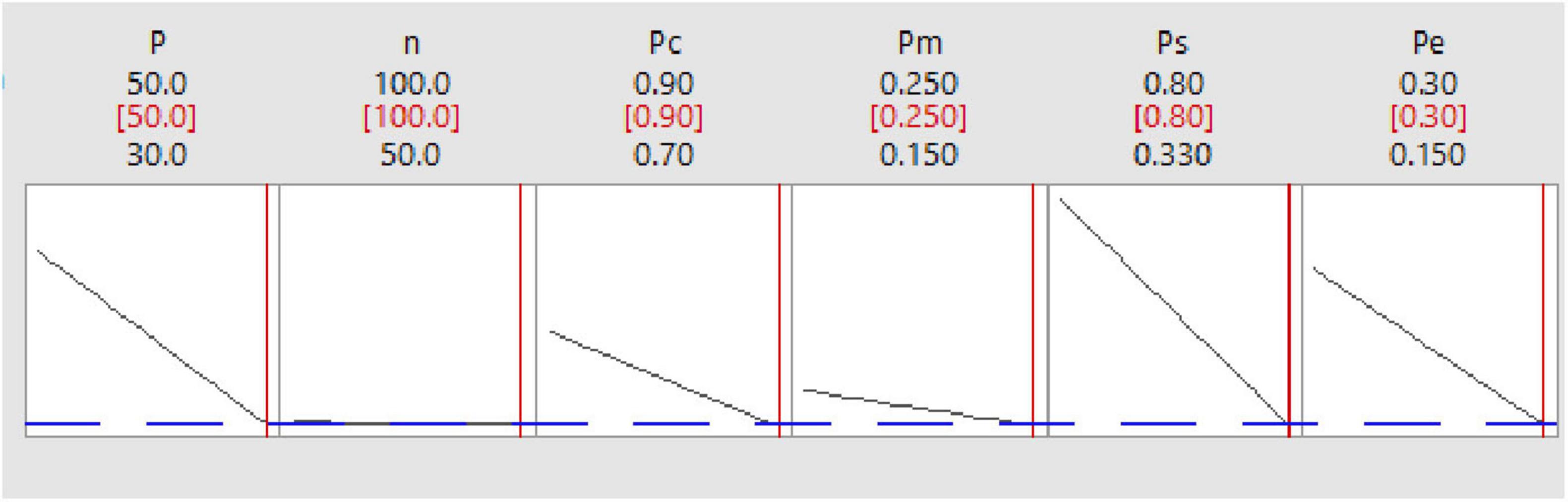
Figure 7. The values of parameters to give the minimum objective value.

P = 50; n = 100; P_{c} = 0.9; P_{m} = 0.25; P_{s} = 0.8; P_{e} = 0.3

The multivariate experiment

A multivariate experiment is conducted with the three affected factors P, P_s, and P_e. The levels of the input factors are chosen as in Table 6.

TABLE 6

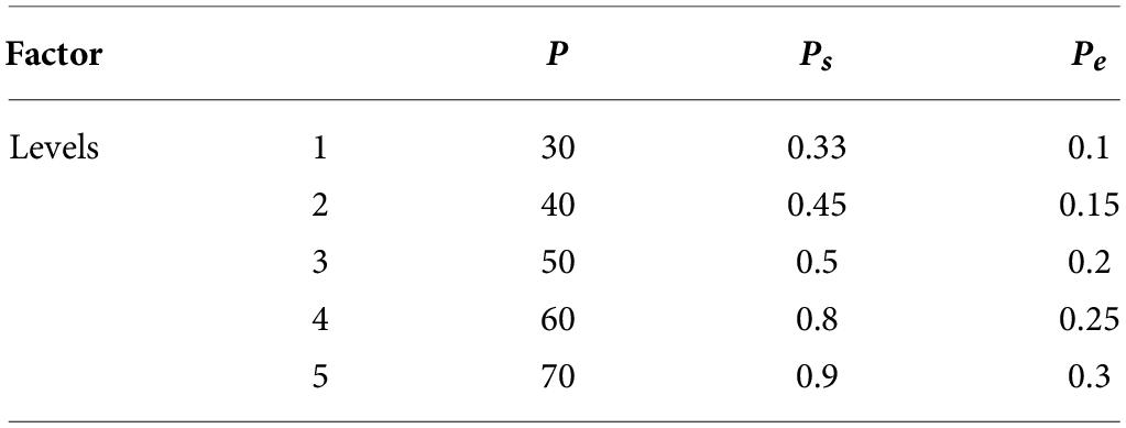
Table 6. Five levels of the input factors.

There are 125 combinations of input factors. With a sample size of 3, the total number of experiments is 375. The experimental results are collected. From the data, the optimized values of parameters are shown in Figure 8.

FIGURE 8

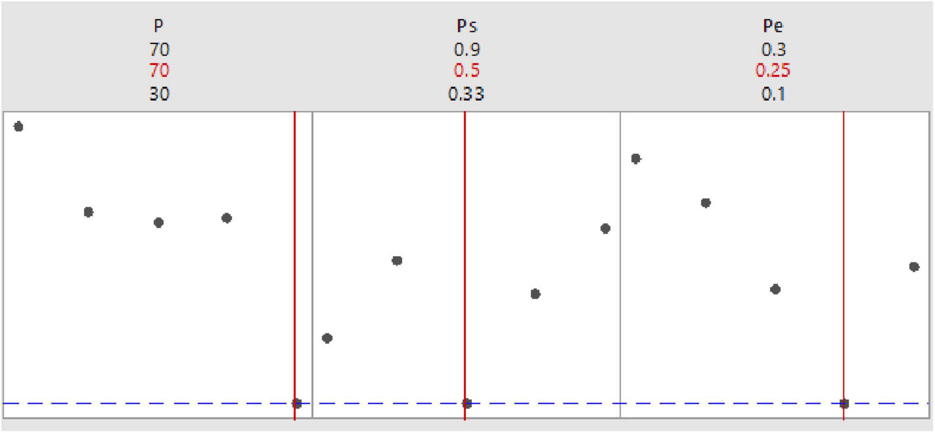
Figure 8. The values of parameters to give the minimum objective value.

The GA model with DOE is run with the parameters defined by the experiment. The objective function is as in Figure 9.

FIGURE 9

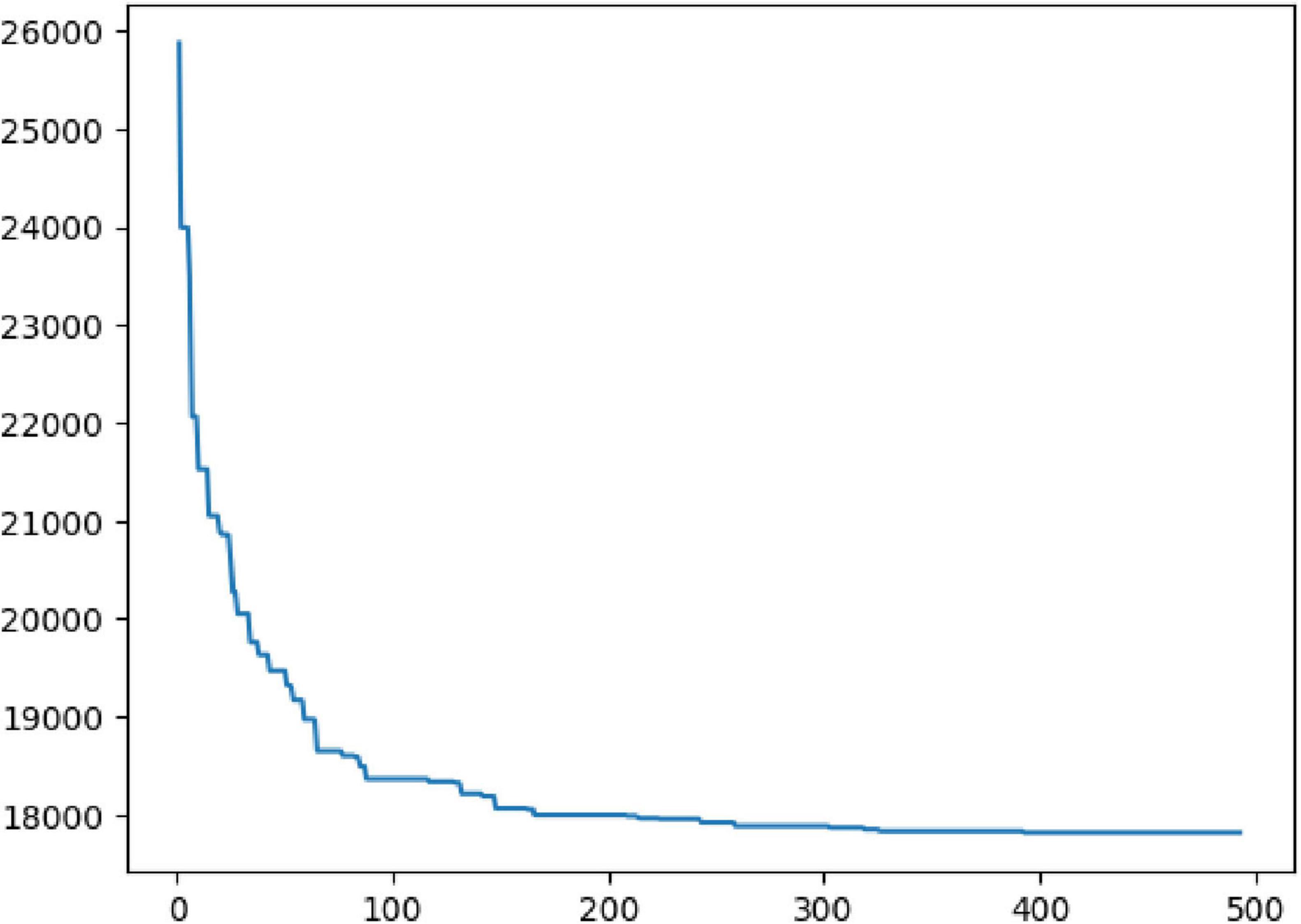
Figure 9. The result of the objective function of the GA model with design of experiment (DOE).

The results of the GA model with DOE are shown as:

Q = | \begin{matrix} 9 & 0 & 0 & 0 & 9 & 0 & 0 & 0 & 4 & 4 & 0 & 2 \\ 6 & 4 & 5 & 0 & 2 & 5 & 6 & 8 & 9 & 2 & 2 & 7 \\ 4 & 4 & 7 & 0 & 6 & 2 & 6 & 0 & 0 & 6 & 0 & 0 \end{matrix} |

With objective value is 17, 816.925.

Table 7 presents the comparison results between the current heuristic method, the GA algorithm, and the GA with DOE.

TABLE 7

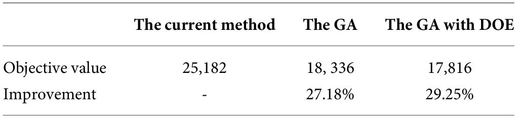
Table 7. Comparison of results.

Conclusion

The dynamic inventory planning problem has been modeled. The GA algorithm has been used to solve this mathematical model. The solution of the GA algorithm is better than the solution of the currently used empirical algorithm. However, it is still a suboptimal solution.

The experimental design is used to optimize the parameters of the GA algorithm. The solution of the GA algorithm with DOE is better than the solution of the GA algorithm. However, the algorithms are only used to solve the pilot problem with three items. The future development direction is for real problems with many items.

Funding

The authors declare that no financial support was received for the research, authorship, and/or publication of this article.

Conflict of interest

The authors declare that the research was conducted in the absence of any commercial or financial relationships that could be construed as a potential conflict of interest.

References

1. Arrow KJ, Harris T, Marschak J. Optimal inventory policy. Econometrica. (1951) 19(3):250–72.

Google Scholar

2. Dvoretzky A, Kiefer J, Wolfowitz J. The inventory problem: I. Case of known distributions of demand. Econometrica. (1952) 20(2):187–222.

Google Scholar

3. Dvoretzky A, Kiefer J, Wolfowitz J. The inventory problem: II. Case of unknown distributions of demand. Econometrica. (1952) 20(3):450–66.

Google Scholar

4. Aggarwal SC. A review of current inventory theory and its applications. Int J Prod Res. (1974) 12(4):443–82.

Google Scholar

5. Mondal S, Maiti M. Multi-item fuzzy EOQ models using genetic algorithm. Comput Indust Eng. (2002) 44(1):105–17.

Google Scholar

6. Maiti MK, Maiti M. Production policy for damageable items with variable cost function in an imperfect production process via genetic algorithm. Math Comput Model. (2005) 42(9–10):977–90.

Google Scholar

7. Pasandideh SHR, Niaki STA, Hajipour V. A multi-objective facility location model with batch arrivals: two parameter-tuned meta-heuristic algorithms. J Intell Manufact. (2011) 24:331–48.

Google Scholar

8. Pasandideh SHR, Niaki STA. A genetic algorithm approach to optimize a multi-products EPQ model with discrete delivery orders and constrained space. Appl Math Comput. (2008) 195(2):506–14.

Google Scholar

9. Tsai MW, Hong TP, Lin WT. A two-dimensional genetic algorithm and its application to aircraft scheduling problem. Math Prob Eng. (2015) 2015:1–15.

Google Scholar

© The Author(s). 2026 Open Access This article is distributed under the terms of the Creative Commons Attribution 4.0 International License (https://creativecommons.org/licenses/by/4.0/), which permits unrestricted use, distribution, and reproduction in any medium, provided you give appropriate credit to the original author(s) and the source, provide a link to the Creative Commons license, and indicate if changes were made.

Application of genetic algorithm (GA) and design of experiment (DOE) to solve the inventory dynamic lot-sizing problem: a case study

Introduction

Literature review & research methodology

Literature review

Inventory dynamic lot-sizing

Genetic algorithm

Research methodology

Mathematical model of the dynamic lot-sizing problem

Assumptions

Parameters

Decision variables

Objective function

Constraints

The GA model for solving the dynamic lot-sizing problem

The method of coding

The GA procedure

Applying the GA model for solving the DLS problem

The GA parameters & factors

The GA operators

The selection operator

The crossover operator

The mutation operator

The replacing operator

The stopping criterion

Applying the GA with DOE to solve the DLS problem

The 2k experiment

The multivariate experiment

Conclusion

Funding

Conflict of interest

References

The 2^k experiment