Visualization of multidimensional areas of solutions to mathematical models of complex objects

Introduction

Algorithms artificial and computational intelligence systems (as subsets of it) use mathematical models related to the search for hidden patterns in incomplete data, pattern recognition and decision-making under uncertainty (1–6). For example, the book by M.T. Jones (5) is devoted to the methods of developing “smart” algorithms. The monograph, which has become a “classic of the genre” (6), presents modern achievements and ideas that have been formulated in the research of many recent years, which have become an incentive for the development of artificial intelligence.

When solving such problems, algorithms for visualizing objects may be needed, mathematical models of which may not have an explicit description (solutions of systems of nonlinear equations, etc.). The simplest stationary models of such objects can be described by algebraic polynomial equations (7) relating to various subject areas of science (engineering, physics, chemistry, and biology) (8–12). When the degree of a polynomial is higher than four, the solutions of even such equations cannot be expressed exactly, but it is known that the number of solutions (roots) of such equations in the complex domain is equal to the degree of the polynomial (the main theorem of algebra) (13).

In general, mathematical models of objects in the space Rⁿ cannot be presented explicitly, because their exact solutions are not known or cannot be expressed in a constructive form (14). In this regard, it is of interest to study the evolution of projections of solutions of multidimensional models of objects of various geometric structures. In practice, the projections located in a certain area of visibility of the image recognition system (accessibility zone, physicality) are of the greatest interest.

The informative value of visualization depends on the direction of designing the coordinate representation on the parameter space. Depending on the chosen direction of design, two qualitatively different areas of the object image (uniqueness and multiplicity) can be distinguished. In the domain of multiplicity, each point has several prototypes, corresponds to several (isolated) points of the original model.

In the area of uniqueness, the various points of the original model remain different, do not mix with each other. The area of multiplicity, if it exists, is an objective disadvantage of choosing the direction of design, because the parameters of the original model cannot be unambiguously restored by the projection parameters. Let’s call the direction of design, in which the area of multiplicity is not empty, the direction of ambiguity.

The mathematical model of any nonlinear object admits multiplicity with a certain choice of design direction. Under certain conditions, there may be such design directions (directions of unambiguity) that each line of this direction intersects with the coordinate representation of the model at no more than one point. The purpose of the article is to create a method for finding the directions of unambiguity of design for models given a surface in Euclidean space.

Research elaborations

Let’s consider the area (domain) of the multiplicity of solutions of polynomial equations with parameters from the point of view of an intelligent pattern recognition system. The most informative (3D) visual representation of this area can be synthesized in the form of projections of some multidimensional object along some direction. If the model admits the existence of a domain of ambiguity with some choice of design direction, then such a choice leads to the so-called “hidden multiplicity.” For this model, with such a choice of direction, it is impossible to restore the original model unambiguously according to the given values of the model parameters, i.e., some points of the original model are “stuck together”, represented as the same value. The model with ambiguity, after such a design, turned into an unambiguous model.

Consider the feasibility of hidden multiplicity on the example of a model with one phase variable x, the stationarity equation of which is the sum of several homogeneous components, each of which is a polynomial of some degree n with coefficients a₀,…,a_n, depending on the parameters of model (0 < x < 1):

The stationary state (SS) is the root of function (1). For example, the function x(1−x)−2/9, of two homogeneous components x(1−x) И/−2/9 has two SS $(x,1-x)=(\frac{1}{3},\frac{2}{3})\text{ and}(\frac{2}{3},\frac{1}{3})$.

To measure the parameters of the model, a certain function is used, which can also be represented by the sum of homogeneous polynomials of degree m (these degrees may not coincide with the degrees of uniformity of the n stationary equation)

For example, the function g(x) = x²(1−x)² takes the same meaning in two SS $(x,1-x)=(\frac{1}{3},\frac{2}{3})$ and $(\frac{2}{3},\frac{\mathrm{\hspace{0.25em}1}}{\mathrm{\hspace{0.25em}3}})$for any parameter values. This means that the multiplicity exists, but it is hidden and cannot be observed on the graph of the dependence of g(x) on any of the parameters.

Let’s find the conditions under which the multiplicity becomes hidden. To do this, it is enough that when replacing x → 1 − x, the function g(x)does not change the value, and the function f(x) retains the module:

Indeed, when executing (3), the function f(x), if it has a root x₀, then it also has a root 1−x₀, i.e., there is a MSS. In this case, the function g(x) in both of these SS has the same value, i.e., the multiplicity is hidden. Note that the functions g(x) (and the functions f(x) in (3), when choosing the plus sign) satisfying (3) are returnable (palindromic), i.e., the list of their coefficients, read from right to left and from left to right, is the same. For example, if we write condition (3) for the polynomial g(x), then the monomes symmetric with respect to the beginning and end will move into each other (swap places), leaving the value of the polynomial unchanged by b_m−p = b_p (the reversibility of the polynomial):

By b_m−p = b_p (the reversibility of the polynomial). For the polynomial f(x), this is also true when choosing the plus sign in (3). If the minus sign in (3) is selected, then the polynomial f(x) will be anti-returnable

on condition a_m−p = −a_p. Thus, for the occurrence of latent multiplicity, it is sufficient to fulfill the conditions of symmetry of the coefficients for monomials of polynomials (2) and (3):

The conditions (4) also apply to functions having several homogeneous components. For specific objects, conditions (4) are equality-type conditions on parameters. This means that hidden multiplicity will occur when visualizing such objects, not in the entire space of acceptable parameter values but on some surface in this space. Hiding is related to the geometry of this surface and the “unsuccessful” choice of the direction of movement along the surface while remaining on it.

There is also a deeper and more common cause of latent multiplicity: “flat” phase multiplicity. Some design directions (directions of unambiguity) may have the property that any straight line in this direction intersects the surface of the model at no more than one point. If such a direction exists for a model that admits multiplicity, then the parameters of this initial model cannot be restored unambiguously.

Let’s consider the geometry of the multiplicity in the example of a polynomial with two homogeneous components:

This is the equation of some surface in a 4D space, where the 3D abscissa axis consists of three parameters k₁, k₋₁, and k₂, and the 1D ordinate axis is the value of x (the objective function). The projection of this surface onto the abscissa axis represents the domain of admissibility—the set of positive values k₁, k₋₁, and k₂, for which the equation of stationarity has at least one solution x. The domain of multiplicity is a part of the domain of admissibility in which each point has at least two prototypes—two different points of the surface, projections projected onto this point.

Let’s find the geometric shape of the areas of acceptability and multiplicity for this example, assuming that the parameters take only positive physical values and the phase variable x varies in the range from 0 to 1 (dimensionless). Then in the band 0 < x < 1, we need to find the intersection of the domain of admissibility and the domain of multiplicity with a positive octant k₁ > 0, k₋₁ > 0, k₂ > 0. Since the function (5) has a value of k₁ > 0 at zero and −k₋₁ < 0 at one, then, being continuous, it must take a 0 value at the interval 0 < x < 1, at least at one point of this interval. This means that the area of validity coincides with all octants. In other words, for any positive values of the parameters, there is at least one stationary state.

The multiplicity domain is characterized by the presence of two or more solutions of equation (5) in the unit interval. For the multiplicity of solutions of the equation f(x) = 0, where f(x) is a continuously differentiable function with the conditions f(0) > 0 > f(1), it is necessary and sufficient that in this interval there exists such a root x₀ of function f(x) in which the derivative is positive or equal to zero:

Condition (6) is a multiplicity criterion for objects described by one independent phase variable. There is no explicit analog of this criterion for multidimensional objects. In our case, in the interval (0, 1) there are one or three roots x₀, x1, x2 (we can assume that x₀ is the middle root 0 < x₁ < x₀ < x₂ < 1). Then, the multiplicity criterion (6) takes the form (0 < x₀ < 1):

Results

The informativeness of the visualization of multiplicity depends on the coordinate representation of the model and the direction of its design on the parameter space. Some directions allow you to hide the multiplicity. Each straight line of such a “correct” direction of unambiguity intersects the coordinate representation of the model at no more than one point. We present a method for finding such design directions for areas of multiple surfaces in Euclidean space.

Parametrization in 3D parameter space (a₁, a₋₁, x₀)

We express k₁ from the equation in the relations (7) and substitute it into the inequality, we get:

Relation (8) distinguishes a surface in 4D space (k₁, k₋₁, k₂, x₀), and (9)—its projection on the 3D axis of the abscissa (k₋₁, k₂, x₀). In this case, k₁ is a 1D ordinate axis. The dimension can be reduced if, instead of the parameters k₁, k₋₁, k₂, we go to the relative values a₁ = k₁/k₂, a₂ = k₋₁/k₂. Then the projection of the model onto the domain (a₁, a₋₁, x₀) appears as the equation of a 2D surface in 3D space

parameterized by two parameters (a₋₁, x₀), varying within the following limits

Relation (11) distinguishes that part of the projection, which is the area of multiplicity.

The formulas for the extreme roots x₁, x2 have the form:

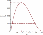
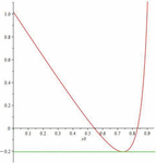
We exclude the parameter x₀ in the relations (10, 11), i.e., we find the projection of the multiplicity domain on the plane (a₋₁, a₁). For a fixed value a_–1, the value x₀ changes in the interval 1/2 < x₀ < 1 so that the inequality a₋₁ ≥ (2x₀−1)(1−x₀)² is satisfied. Graph of the function max⁡(a₋₁) = (2x₀−1)(1−x₀)² in the interval 1/2 < x₀ < 1 is shown in Figure 1. For a fixed (within 0 < a₋₁ ≥ 1/27) value of a_–1 the parameter a₁ takes the value described by formula (10), where x₀ changes occur in some interval within the segment [1/2, 1], which depends on the selected value of a_–1. In Figure 1, this interval is shown when a₋₁ = 0.01. The derivative of a₁, which is a function (10) of x₀, has the form:

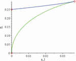
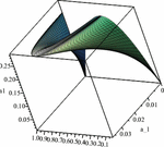
This derivative, taking into account (10), is not positive in the parameter domain under consideration. Therefore, with a fixed a_–1, the value of a₁, as a function of x₀, monotonically decreases, taking values on a certain segment. Thus, on the plane (a₋₁, a₁), the projection of the multiplicity domain looks as shown in Figure 2. For the lower and upper branches of the projection of the multiplicity domain onto the plane (a₋₁, a₁), exact equations can be obtained, but due to their cumbersomeness, we do not give them here. The surface of stationary states as a whole is all three roots together on one graph in the space (a–1, a1, x), as shown on Figure 3.

The stationary surface of the model given by equation (5) is a 2D manifold in space (a–1, a1, x). It has three branches and can be described through the parameters (a_–1, x₀) using three local maps (coordinate systems): average a₋₁ = a₋₁, $a_1=\frac{a_{-1}{x}_0}{1-x_0}+x_0(1-x_0)$, x = x₀,lower a₋₁ = a₋₁, $a_1=\frac{a_{-1}{x}_0}{1-x_0}+x_0(1-x_0)$, $x=1-\frac{1}{2}{x}_0\left(1+\sqrt{1-\frac{4a_{-1}}{x_0{}^2\left(1-x_0\right)}}\right),$upper a₋₁ = a₋₁, $a_1=\frac{a_{-1}{x}_0}{1-x_0}+x_0(1-x_0)$, $x=1-\frac{1}{2}{x}_0\left(1-\sqrt{1-\frac{4a_{-1}}{x_0{}^2\left(1-x_0\right)}}\right).$ These branches are located above the area 0 < a₋₁ = (2x₀−1)(1−x₀)², 1/2 < x₀ < 1. The middle branch merges with the lower one at a₋₁ = (2x₀−1)(1−x₀)², 1/2 < x₀ = 2/3. The middle branch merges with the upper one at a₋₁ = (2x₀−1)(1−x₀)², $\frac{2}{3}=x_0<1.$ All three branches merge when a₋₁ = 1/27, a₁ = 8/27, x₀ = 2/3.

Note that (10, 11) contain a non-strict inequality, and it may seem that this variety has an edge, which, if it exists, is a line:

We show that this manifold has no edge. To do this, we will choose a substitution of variables in which our manifold will be diffeomorphic to the plane. This is achieved by a combination of two techniques.

A non-strict inequality of the form g ≤ 0 is replaced by the equation g = p², where p is a new variable. A strict inequality of the form g > 0 is replaced by the equation g = e^p. In each of these cases, the dimension of the model and the number of equations increase by 1.

The double inequality 0 < g < 1 leads to two new equations g = e^p, e^p + e^q = 1, including two new variables p, q whose values are arbitrary. We apply these transformations to the relations (10) and (11) and obtain the following representation of the multiplicity domain:

Thus, the multiplicity domain is a 2D manifold in space (a₁, p₋₁, x₀, p₂, p₃, p₄). At the same time, there are no restrictions on these six variables. The expression of four of the variables through the other two (p₂, p₃) shows

that the region of multiplicity is mutually unambiguously mapped to the plane (p₂, p₃).

Choosing the “right” direction of design

Let’s be given some equations of a stationary surface f(x) = 0 in space (x). Let’s consider all the projections of this surface in the direction of some design vector (ε) and the orthogonal design plane to it. By shifting this plane along the projection vector, if necessary, we can consider it a tangent plane to a stationary surface at some point (x₀).

It is obvious that if the design, with its chosen direction, is reversible (i.e., the prototype of each projection point is unique) on the entire projection area, then it must be reversible and locally, in the neighborhood of the point (x₀). It is also obvious that the projection is locally reversible only if it is directed along the gradient $f{}^{\prime }\left(x\right)$ of the function. Thus, among all the directions of design locally, in the vicinity of the point (x₀), only design in one direction is reversible; all the others lead to ambiguity.

This locally reversible design may or may not be globally reversible (only in this case the graph of a stationary surface above the design plane be characterized by uniqueness). However, a globally reversible design must be locally reversible at every point on the surface.

Local multiplicity

The points of the surface at which the condition of local reversibility is violated are called points of local multiplicity. They are characterized by the following condition: the orthogonal complement to the tangent plane at the point of the surface x₀ must have a non-empty intersection with the tangent plane at some other point of the surface x₁. In the special case when the orthogonal complement has dimension 1 (i.e., when the normal to the surface is uniquely determined, in other words, when the surface is a hypersurface, i.e., has codimension 1), this condition means the orthogonality of the normals to the surface at these two points x₀, x₁. In this case, both points are points of local multiplicity. Such points always appear in pairs. The points for which the pair is not found are points of local reversibility. The normal to such a point determines the direction of a locally reversible projection.

For example, the surface k−x² = 0 on the plane (x, k) is an ordinary parabola. The normal to the surface is uniquely determined; it is a vector (−2x,1). The local multiplicity condition (−2x₀)*(−2x₁) + 1*1 = 0 takes the form 4x₀x₁ + 1=0. As you can see, two points of the surface (x₀, k₀), (x₁, k₁) enter this condition equally, symmetrically. This condition is met for any values of x₀, except zero. The origin of coordinates x₀ = 0, k₀ = 0 is the only point of local unambiguity. The gradient at this point, equal to (0, 1), determines the only direction (upward) of the locally reversible projection.

Similarly, for a surface k−xz = 0,x + z = 1 in space (x, z, k) (projected onto the plane (x, k), it is the same parabola, but shifted: k = x(1−x) the orthogonal complement is 2D; it is the plane of gradients (z,−x,1), (1, 1, 0). The tangent plane is 1D and is given by the vector (1,−1,z–x), orthogonal gradients. This vector (1,−1,zz₀−x₀) at one of the points (x₀, z₀, k₀) should be orthogonal to the gradients (rz₁,−x₁,1), (1, 1, 0) at the other point (x₁, z₁, k₁). Orthogonality condition is x₁−z₁ = x₀−z₀. Expressing z by x, we get x₁ = x₀. The point x₀ = 1/2,z₀ = 1/2, k₀ = 1/4 is the only point of local unambiguity. Direction (1, s the) is the only direction of locally reversible design.

As a rule, and in general, almost all points on the surface are points of local multiplicity. The points of local unambiguity and, accordingly, the directions of locally reversible design constitute a set of codimensions 1 and higher, or may even be isolated points, as in the two examples discussed aearlier.

For the surface az−b (1−z) − z² (1−z) = 0 considered in space (a, b, z), corresponding to the model (10) (we slightly changed the notation of variables by removing the indexes), the gradient is (z, z−1, a + b−2z + 3z²). The condition of orthogonality of gradients at two different points (a₁, b₁, z₁), (a₂, b₂, z₂) has the following form: $z_1{z}_2+\left(1-z_1\right)\left(1-z_2\right)+\left(a_1+b_1-2z_1+3z_1{}^2\right)\left(a_2+b_2-2z_2+3z_2{}^2\right)=0$. Taking into account the relations $a_1+b_1=\frac{b_1}{z_1}+z_1\left(1-z_1\right)$, $a_2+b_2=\frac{b_2}{z_2}+z_2\left(1-z_2\right)$, that are fulfilled on the surface, the orthogonality condition can be reduced to the form $z_1{z}_2+\left(1-z_1\right)\left(1-z_2\right)+(\frac{b_1}{z_1}-z_1\left(1-2z_1\right))(\frac{b_2}{z_2}-z_2\left(1-2z_2\right))=0$. The first two terms are positive, so one of the brackets, let the first one, should be positive, the other negative. Therefore, $b_1>z_1{}^2\left(1-2z_1\right)$, z₂ < 1/2 И/$b_2<z_2{}^2\left(1-2z_2\right)$. Let us further assume that these inequalities are fulfilled. With fixed z₂, b₂ within these limits, the right part of the expression

accepts all negative values, with the appropriate selection of z₁, b₁. Thus, the points of local multiplicity (a₂, b₂, z₂) are described by the relations

All other points on the surface are points of local reversibility. Gradients at these points are directions of locally unambiguous design.

A design that hides multiplicity

We can determine the direction of design (the direction of unambiguity), hiding multiplicity, based on the following considerations. Let there be a function y = f(x), differentiable in a connected convex domain D of the space Rⁿ. We are looking for the “right” direction of the design defined by the vector d, such that each of the lines of the family y = dx + c intersects the graph of the function f(x) at no more than one point. We formulate a condition for the “correct” vector d.

Criteria

The directions of unambiguity are in addition to the set of directions of the gradients of the function under study, calculated at all points of the domain D.

Proof

If any of these lines intersect the graph twice, say, at points x = a and x = b, then according to Lagrange’s mean value theorem, there is a point c on the segment [a, b] in which the tangent is parallel to the chord connecting the points [a, f(a)] and [b, f(b)]. In other words, the normal of the segment coincides with the gradient of the function f(x) at some point c of the segment. Thus, the vector d coinciding with the gradient of the function f at some point in the domain D cannot be the direction of unambiguity. The opposite is also true: any direction that does not coincide with the gradient of the function f at any point in the domain D is the direction of unambiguity.

Examples of the application of the criterion of directions of unambiguity

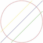
Example 1. The circle x² + y² = 1 preserves multiplicity in any direction of design (Figure 4).

Example 2. The parabola y = x² on the unit segment 0 ≤ x ≤ 1 allows hiding multiplicity. Its gradient 2x takes values on the segment [0, 2]. Therefore, the design direction y = dx hides multiplicity at d < 0 or d > 2 (Figures 5A, C).

Example 3. Bell. The function y = 1/(1 + 5x²), considered on the entire numerical axis, also allows hiding multiplicity with a suitable choice of the design direction. The gradient of this function, −10x/(1 + 5x²)², takes values on the segment [mn = −(3√15)/8, mx = 3√15)/8]. Therefore, the correct design direction d is determined by the conditions d < mn or d > mx (Figures 6A, C).

Applying the criterion to the model (7)

We apply this method to determining the correct directions for designing the function (10). This function depends on the parameter a_–1 and, at 0 < a₋₁ <1/27, is characterized by multiplicity. The derivative of this function on the segment x = [0, 1] takes values from mn = 3³√a₋₁−1 to mx = +∞ (Figure 7). Therefore, all directions of hidden multiplicity are determined by the inequality d < mn (Figures 8A, B).

Conclusion

Thus, hidden multiplicity (i.e., the existence of unambiguity directions for models that admit multiplicity) occurs quite often, especially if the model is considered not in the entire parameter space but in a certain zone of physicality. The paper presents a criterion that allows finding the directions of unambiguity for a wide class of models. The criterion is illustrated by the example of curves on a plane and surfaces in space defined by a function of the form y = f(x), but it can also be used in the multidimensional case, which can be the subject of further research.

Author contributions

BA: ideas, formulas, and drawings. VF: discussion of the work, text, design, and correspondence with the editors. Both authors contributed to the article and approved the submitted version.

References

4. Kruse R, Borgelt C, Klawonn F, Moewes C, Steinbrecher M, Held P. Computational Intelligence: A Methodological Introduction. London: Springer (2013).
8. Bolshakov AA. Development of an autostereoscopic 3D display for visualization of moving three-dimensional images as part of multimedia and communication equipment. Math Methods Eng Technol MMTT. (2019) 12:40–9.
9. Molochko AV. On the way of expanding the boundaries of perception and visualization of cartographic images. Video Sci. (2019) 14:2–11.
10. Lozhkin LD, Voronoi AA, Ankina KP, et al. Visualization of optical images. Int J Appl Fundament Res. (2019) 1:125–9.
11. Kovtun DR. Application of the method of visualization of image classes in multidimensional feature spaces for the evaluation of technically complex objects. Auditorium. (2014) 1:105–7.
12. Artyushenko VM, Abbasov AE. The use of visualization methods using 3D images for technological processes of assembly and testing of complex technical devices. Modern Technol Syst Anal Modeling. (2015) 48:38–43.